- You are here:
-
Home

-
Contents
-
Part VII. The Environment
- Environmental Pollution Control

55. Environmental Pollution Control
Chapter Editors: Jerry Spiegel and Lucien Y. Maystre
Table of Contents
Tables and Figures
Environmental Pollution Control and Prevention
Jerry Spiegel and Lucien Y. Maystre
Air Pollution Management
Dietrich Schwela and Berenice Goelzer
Air Pollution: Modelling of Air Pollutant Dispersion
Marion Wichmann-Fiebig
Air Quality Monitoring
Hans-Ulrich Pfeffer and Peter Bruckmann
Air Pollution Control
John Elias
Water Pollution Control
Herbert C. Preul
Dan Region Sewage Reclamation Project: A Case Study
Alexander Donagi
Principles of Waste Management
Lucien Y. Maystre
Solid Waste Management and Recycling
Niels Jorn Hahn and Poul S. Lauridsen
Case Study: Canadian Multimedia Pollution Control and Prevention on the Great Lakes
Thomas Tseng, Victor Shantora and Ian R. Smith
Cleaner Production Technologies
David Bennett
Tables
Click a link below to view table in article context.
1. Common atmospheric pollutants & their sources
2. Measurement planning parameters
3. Manual measurement procedures for inorganic gases
4. Automated measurement procedures for inorganic gases
5. Measurement procedures for suspended particulate
6. Long-distance measurement procedures
7. Chromatographic air quality measurement procedures
8. Systematic air quality monitoring in Germany
9. Steps in selecting pollution controls
10. Air quality standards for sulphur dioxide
11. Air quality standards for benzene
12. Examples of best available control technology
13. Industrial gas: cleaning methods
14. Sample emission rates for industrial processes
15. Wastewater treatment operations & processes
16. List of investigated parameters
17. Parameters investigated at the recovery wells
18. Sources of waste
19. Criteria for selection of substances
20. Reductions in releases of dioxin & furan in Canada
Figures
Point to a thumbnail to see figure caption, click to see figure in article context.
|
|


Environmental Pollution Control and Prevention
Over the course of the twentieth century, growing recognition of the environmental and public health impacts associated with anthropogenic activities (discussed in the chapter Environmental Health Hazards) has prompted the development and application of methods and technologies to reduce the effects of pollution. In this context, governments have adopted regulatory and other policy measures (discussed in the chapter Environmental Policy) to minimize negative effects and ensure that environmental quality standards are achieved.
The objective of this chapter is to provide an orientation to the methods that are applied to control and prevent environmental pollution. The basic principles followed for eliminating negative impacts on the quality of water, air or land will be introduced; the shifting emphasis from control to prevention will be considered; and the limitations of building solutions for individual environmental media will be examined. It is not enough, for example, to protect air by removing trace metals from a flue gas only to transfer these contaminants to land through improper solid waste management practices. Integrated multimedia solutions are required.
The Pollution Control Approach
The environmental consequences of rapid industrialization have resulted in countless incidents of land, air and water resources sites being contaminated with toxic materials and other pollutants, threatening humans and ecosystems with serious health risks. More extensive and intensive use of materials and energy has created cumulative pressures on the quality of local, regional and global ecosystems.
Before there was a concerted effort to restrict the impact of pollution, environmental management extended little beyond laissez-faire tolerance, tempered by disposal of wastes to avoid disruptive local nuisance conceived of in a short-term perspective. The need for remediation was recognized, by exception, in instances where damage was determined to be unacceptable. As the pace of industrial activity intensified and the understanding of cumulative effects grew, a pollution control paradigm became the dominant approach to environmental management.
Two specific concepts served as the basis for the control approach:
- the assimilative capacity concept, which asserts the existence of a specified level of emissions into the environment which does not lead to unacceptable environmental or human health effects
- the principle of control concept, which assumes that environmental damage can be avoided by controlling the manner, time and rate at which pollutants enter the environment
Under the pollution control approach, attempts to protect the environment have especially relied on isolating contaminants from the environment and using end-of-pipe filters and scrubbers. These solutions have tended to focus on media-specific environmental quality objectives or emission limits, and have been primarily directed at point source discharges into specific environmental media (air, water, soil).
Applying Pollution Control Technologies
Application of pollution control methods has demonstrated considerable effectiveness in controlling pollution problems - particularly those of a local character. Application of appropriate technologies is based on a systematic analysis of the source and nature of the emission or discharge in question, of its interaction with the ecosystem and the ambient pollution problem to be addressed, and the development of appropriate technologies to mitigate and monitor pollution impacts.
In their article on air pollution control, Dietrich Schwela and Berenice Goelzer explain the importance and implications of taking a comprehensive approach to assessment and control of point sources and non-point sources of air pollution. They also highlight the challenges - and opportunities - that are being addressed in countries that are undergoing rapid industrialization without having had a strong pollution control component accompanying earlier development.
Marion Wichman-Fiebig explains the methods that are applied to model air pollutant dispersion to determine and characterize the nature of pollution problems. This forms the basis for understanding the controls that are to be put into effect and for evaluating their effectiveness. As the understanding of potential impacts has deepened, appreciation of effects has expanded from the local to the regional to the global scale.
Hans-Ulrich Pfeffer and Peter Bruckmann provide an introduction to the equipment and methods that are used to monitor air quality so that potential pollution problems can be assessed and the effectiveness of control and prevention interventions can be evaluated.
John Elias provides an overview of the types of air pollution controls that can be applied and the issues that must be addressed in selecting appropriate pollution control management options.
The challenge of water pollution control is addressed by Herbert Preul in an article which explains the basis whereby the earth’s natural waters may become polluted from point, non-point and intermittent sources; the basis for regulating water pollution; and the different criteria that can be applied in determining control programmes. Preul explains the manner in which discharges are received in water bodies, and may be analysed and evaluated to assess and manage risks. Finally, an overview is provided of the techniques that are applied for large-scale wastewater treatment and water pollution control.
A case study provides a vivid example of how wastewater can be reused - a topic of considerable significance in the search for ways that environmental resources can be used effectively, especially in circumstances of scarcity. Alexander Donagi provides a summary of the approach that has been pursued for the treatment and groundwater recharge of municipal wastewater for a population of 1.5 million in Israel.
Comprehensive Waste Management
Under the pollution control perspective, waste is regarded as an undesirable by-product of the production process which is to be contained so as to ensure that soil, water and air resources are not contaminated beyond levels deemed to be acceptable. Lucien Maystre provides an overview of the issues that must be addressed in managing waste, providing a conceptual link to the increasingly important roles of recycling and pollution prevention.
In response to extensive evidence of the serious contamination associated with unrestricted management of waste, governments have established standards for acceptable practices for collection, handling and disposal to ensure environmental protection. Particular attention has been paid to the criteria for environmentally safe disposal through sanitary landfills, incineration and hazardous-waste treatment.
To avoid the potential environmental burden and costs associated with the disposal of waste and promote a more thorough stewardship of scarce resources, waste minimization and recycling have received growing attention. Niels Hahn and Poul Lauridsen provide a summary of the issues that are addressed in pursuing recycling as a preferred waste management strategy, and consider the potential worker exposure implications of this.
Shifting Emphasis to Pollution Prevention
End-of-pipe abatement risks transferring pollution from one medium to another, where it may either cause equally serious environmental problems, or even end up as an indirect source of pollution to the same medium. While not as expensive as remediation, end-of-pipe abatement can contribute significantly to the costs of production processes without contributing any value. It also typically is associated with regulatory regimes which add other sets of costs associated with enforcing compliance.
While the pollution control approach has achieved considerable success in producing short-term improvements for local pollution problems, it has been less effective in addressing cumulative problems that are increasingly recognized on regional (e.g., acid rain) or global (e.g., ozone depletion) levels.
The aim of a health-oriented environmental pollution control programme is to promote a better quality of life by reducing pollution to the lowest level possible. Environmental pollution control programmes and policies, whose implications and priorities vary from country to country, cover all aspects of pollution (air, water, land and so on) and involve coordination among areas such as industrial development, city planning, water resources development and transportation policies.
Thomas Tseng, Victor Shantora and Ian Smith provide a case study example of the multimedia impact that pollution has had on a vulnerable ecosystem subjected to many stresses - the North American Great Lakes. The limited effectiveness of the pollution control model in dealing with persistent toxins that dissipate through the environment is particularly examined. By focusing on the approach being pursued in one country and the implications that this has for international action, the implications for actions that address prevention as well as control are illustrated.
As environmental pollution control technologies have become more sophisticated and more expensive, there has been a growing interest in ways to incorporate prevention in the design of industrial processes - with the objective of eliminating harmful environmental effects while promoting the competitiveness of industries. Among the benefits of pollution prevention approaches, clean technologies and toxic use reduction is the potential for eliminating worker exposure to health risks.
David Bennett provides an overview of why pollution prevention is emerging as a preferred strategy and how it relates to other environmental management methods. This approach is central to implementing the shift to sustainable development which has been widely endorsed since the release of the United Nations Commission on Trade and Development in 1987 and reiterated at the Rio United Nations Conference on Environment and Development (UNCED) Conference in 1992.
The pollution prevention approach focuses directly on the use of processes, practices, materials and energy that avoid or minimize the creation of pollutants and wastes at source, and not on “add-on” abatement measures. While corporate commitment plays a critical role in the decision to pursue pollution prevention (see Bringer and Zoesel in Environmental policy), Bennett draws attention to the societal benefits in reducing risks to ecosystem and human health—and the health of workers in particular. He identifies principles that can be usefully applied in assessing opportunities for pursuing this approach.
Air Pollution Management
Air pollution management aims at the elimination, or reduction to acceptable levels, of airborne gaseous pollutants, suspended particulate matter and physical and, to a certain extent, biological agents whose presence in the atmosphere can cause adverse effects on human health (e.g., irritation, increase of incidence or prevalence of respiratory diseases, morbidity, cancer, excess mortality) or welfare (e.g., sensory effects, reduction of visibility), deleterious effects on animal or plant life, damage to materials of economic value to society and damage to the environment (e.g., climatic modifications). The serious hazards associated with radioactive pollutants, as well as the special procedures required for their control and disposal, also deserve careful attention.
The importance of efficient management of outdoor and indoor air pollution cannot be overemphasized. Unless there is adequate control, the multiplication of pollution sources in the modern world may lead to irreparable damage to the environment and mankind.
The objective of this article is to give a general overview of the possible approaches to the management of ambient air pollution from motor vehicle and industrial sources. However, it is to be emphasized from the very beginning that indoor air pollution (in particular, in developing countries) might play an even larger role than outdoor air pollution due to the observation that indoor air pollutant concentrations are often substantially higher than outdoor concentrations.
Beyond considerations of emissions from fixed or mobile sources, air pollution management involves consideration of additional factors (such as topography and meteorology, and community and government participation, among many others) all of which must be integrated into a comprehensive programme. For example, meteorological conditions can greatly affect the ground-level concentrations resulting from the same pollutant emission. Air pollution sources may be scattered over a community or a region and their effects may be felt by, or their control may involve, more than one administration. Furthermore, air pollution does not respect any boundaries, and emissions from one region may induce effects in another region by long-distance transport.
Air pollution management, therefore, requires a multidisciplinary approach as well as a joint effort by private and governmental entities.
Sources of Air Pollution
The sources of man-made air pollution (or emission sources) are of basically two types:
- stationary, which can be subdivided into area sources such as agricultural production, mining and quarrying, industrial, point and area sources such as manufacturing of chemicals, nonmetallic mineral products, basic metal industries, power generation and community sources (e.g., heating of homes and buildings, municipal waste and sewage sludge incinerators, fireplaces, cooking facilities, laundry services and cleaning plants)
- mobile, comprising any form of combustion-engine vehicles (e.g., light-duty gasoline powered cars, light- and heavy-duty diesel powered vehicles, motorcycles, aircraft, including line sources with emissions of gases and particulate matter from vehicle traffic).
In addition, there are also natural sources of pollution (e.g., eroded areas, volcanoes, certain plants which release great amounts of pollen, sources of bacteria, spores and viruses). Natural sources are not discussed in this article.
Types of Air Pollutants
Air pollutants are usually classified into suspended particulate matter (dusts, fumes, mists, smokes), gaseous pollutants (gases and vapours) and odours. Some examples of usual pollutants are presented below:
Suspended particulate matter (SPM, PM-10) includes diesel exhaust, coal fly-ash, mineral dusts (e.g., coal, asbestos, limestone, cement), metal dusts and fumes (e.g., zinc, copper, iron, lead) and acid mists (e.g., sulphuric acid), fluorides, paint pigments, pesticide mists, carbon black and oil smoke. Suspended particulate pollutants, besides their effects of provoking respiratory diseases, cancers, corrosion, destruction of plant life and so on, can also constitute a nuisance (e.g., accumulation of dirt), interfere with sunlight (e.g., formation of smog and haze due to light scattering) and act as catalytic surfaces for reaction of adsorbed chemicals.
Gaseous pollutants include sulphur compounds (e.g., sulphur dioxide (SO2) and sulphur trioxide (SO3)), carbon monoxide, nitrogen compounds (e.g., nitric oxide (NO), nitrogen dioxide (NO2), ammonia), organic compounds (e.g., hydrocarbons (HC), volatile organic compounds (VOC), polycyclic aromatic hydrocarbons (PAH), aldehydes), halogen compounds and halogen derivatives (e.g., HF and HCl), hydrogen sulphide, carbon disulphide and mercaptans (odours).
Secondary pollutants may be formed by thermal, chemical or photochemical reactions. For example, by thermal action sulphur dioxide can oxidize to sulphur trioxide which, dissolved in water, gives rise to the formation of sulphuric acid mist (catalysed by manganese and iron oxides). Photochemical reactions between nitrogen oxides and reactive hydrocarbons can produce ozone (O3), formaldehyde and peroxyacetyl nitrate (PAN); reactions between HCl and formaldehyde can form bis-chloromethyl ether.
While some odours are known to be caused by specific chemical agents such as hydrogen sulphide (H2S), carbon disulphide (CS2) and mercaptans (R-SH or R1-S-R2) others are difficult to define chemically.
Examples of the main pollutants associated with some industrial air pollution sources are presented in table 1 (Economopoulos 1993).
Table 1. Common atmospheric pollutants and their sources
|
Category |
Source |
Emitted pollutants |
|
Agriculture |
Open burning |
SPM, CO, VOC |
|
Mining and |
Coal mining Crude petroleum Non-ferrous ore mining Stone quarrying |
SPM, SO2, NOx, VOC SO2 SPM, Pb SPM |
|
Manufacturing |
Food, beverages and tobacco Textiles and leather industries Wood products Paper products, printing |
SPM, CO, VOC, H2S SPM, VOC SPM, VOC SPM, SO2, CO, VOC, H2S, R-SH |
|
Manufacture |
Phthalic anhydride Chlor-alkali Hydrochloric acid Hydrofluoric acid Sulphuric acid Nitric acid Phosphoric acid Lead oxide and pigments Ammonia Sodium carbonate Calcium carbide Adipic acid Alkyl lead Maleic anhydride and Fertilizer and Ammonium nitrate Ammonium sulphate Synthetic resins, plastic Paints, varnishes, lacquers Soap Carbon black and printing ink Trinitrotoluene |
SPM, SO2, CO, VOC Cl2 HCl HF, SiF4 SO2, SO3 NOx SPM, F2 SPM, Pb SPM, SO2, NOx, CO, VOC, NH3 SPM, NH3 SPM SPM, NOx, CO, VOC Pb CO, VOC SPM, NH3 SPM, NH3, HNO3 VOC SPM, VOC, H2S, CS2 SPM, VOC SPM SPM, SO2, NOx, CO, VOC, H2S SPM, SO2, NOx, SO3, HNO3 |
|
Petroleum refineries |
Miscellaneous products |
SPM, SO2, NOx, CO, VOC |
|
Non-metallic mineral |
Glass products Structural clay products Cement, lime and plaster |
SPM, SO2, NOx, CO, VOC, F SPM, SO2, NOx, CO, VOC, F2 SPM, SO2, NOx, CO |
|
Basic metal industries |
Iron and steel Non-ferrous industries |
SPM, SO2, NOx, CO, VOC, Pb SPM, SO2, F, Pb |
|
Power generation |
Electricity, gas and steam |
SPM, SO2, NOx, CO, VOC, SO3, Pb |
|
Wholesale and |
Fuel storage, filling operations |
VOC |
|
Transport |
SPM, SO2, NOx, CO, VOC, Pb |
|
|
Community services |
Municipal incinerators |
SPM, SO2, NOx, CO, VOC, Pb |
Source: Economopoulos 1993
Clean Air Implementation Plans
Air quality management aims at the preservation of environmental quality by prescribing the tolerated degree of pollution, leaving it to the local authorities and polluters to devise and implement actions to ensure that this degree of pollution will not be exceeded. An example of legislation within this approach is the adoption of ambient air quality standards based, very often, on air quality guidelines (WHO 1987) for different pollutants; these are accepted maximum levels of pollutants (or indicators) in the target area (e.g., at ground level at a specified point in a community) and can be either primary or secondary standards. Primary standards (WHO 1980) are the maximum levels consistent with an adequate safety margin and with the preservation of public health, and must be complied with within a specific time limit; secondary standards are those judged to be necessary for protection against known or anticipated adverse effects other than health hazards (mainly on vegetation) and must be complied “within a reasonable time”. Air quality standards are short-, medium- or long-term values valid for 24 hours per day, 7 days per week, and for monthly, seasonal or annual exposure of all living subjects (including sensitive subgroups such as children, the elderly and the sick) as well as non-living objects; this is in contrast to maximum permissible levels for occupational exposure, which are for a partial weekly exposure (e.g., 8 hours per day, 5 days per week) of adult and supposedly healthy workers.
Typical measures in air quality management are control measures at the source, for example, enforcement of the use of catalytic converters in vehicles or of emission standards in incinerators, land-use planning and shut-down of factories or reduction of traffic during unfavourable weather conditions. The best air quality management stresses that the air pollutant emissions should be kept to a minimum; this is basically defined through emission standards for single sources of air pollution and could be achieved for industrial sources, for example, through closed systems and high-efficiency collectors. An emission standard is a limit on the amount or concentration of a pollutant emitted from a source. This type of legislation requires a decision, for each industry, on the best means of controlling its emissions (i.e., fixing emission standards).
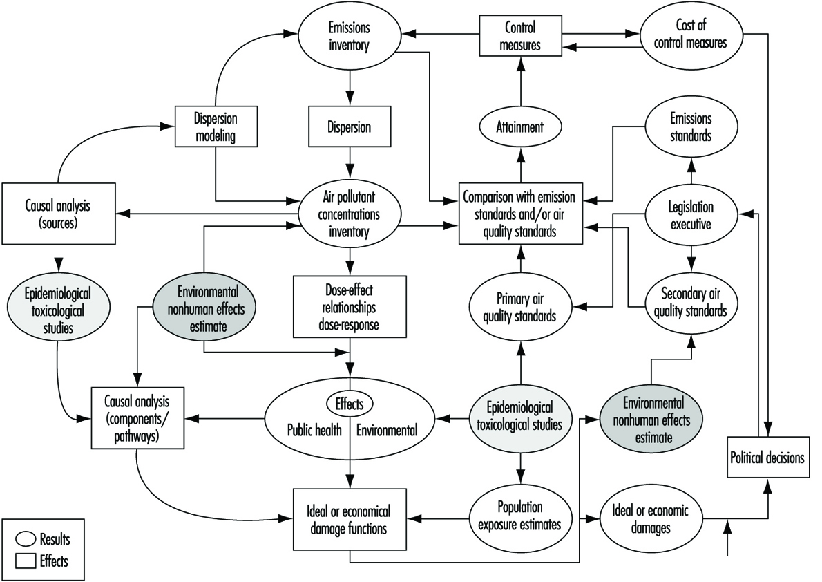
The basic aim of air pollution management is to derive a clean air implementation plan (or air pollution abatement plan) (Schwela and Köth-Jahr 1994) which consists of the following elements:
- description of area with respect to topography, meteorology and socioeconomy
- emissions inventory
- comparison with emission standards
- air pollutant concentrations inventory
- simulated air pollutant concentrations
- comparison with air quality standards
- inventory of effects on public health and the environment
- causal analysis
- control measures
- cost of control measures
- cost of public health and environmental effects
- cost-benefit analysis (costs of control vs. costs of efforts)
- transportation and land-use planning
- enforcement plan; resource commitment
- projections for the future on population, traffic, industries and fuel consumption
- strategies for follow-up.
Some of these issues will be described below.
Emissions Inventory; Comparison with Emission Standards
The emissions inventory is a most complete listing of sources in a given area and of their individual emissions, estimated as accurately as possible from all emitting point, line and area (diffuse) sources. When these emissions are compared with emission standards set for a particular source, first hints on possible control measures are given if emission standards are not complied with. The emissions inventory also serves to assess a priority list of important sources according to the amount of pollutants emitted, and indicates the relative influence of different sources—for example, traffic as compared to industrial or residential sources. The emissions inventory also allows an estimate of air pollutant concentrations for those pollutants for which ambient concentration measurements are difficult or too expensive to perform.
Air Pollutant Concentrations Inventory; Comparison with Air Quality Standards
The air pollutant concentrations inventory summarizes the results of the monitoring of ambient air pollutants in terms of annual means, percentiles and trends of these quantities. Compounds measured for such an inventory include the following:
- sulphur dioxide
- nitrogen oxides
- suspended particulate matter
- carbon monoxide
- ozone
- heavy metals (Pb, Cd, Ni, Cu, Fe, As, Be)
- polycyclic aromatic hydrocarbons: benzo(a)pyrene, benzo(e)pyrene, benzo(a)anthracene, dibenzo(a,h)anthracene, benzoghi)perylene, coronen
- volatile organic compounds: n-hexane, benzene, 3-methyl-hexane, n-heptane, toluene, octane, ethyl-benzene xylene (o-,m-,p-), n-nonane, isopropylbenzene, propylbenezene, n-2-/3-/4-ethyltoluene, 1,2,4-/1,3,5-trimethylbenzene, trichloromethane, 1,1,1 trichloroethane, tetrachloromethane, tri-/tetrachloroethene.
Comparison of air pollutant concentrations with air quality standards or guidelines, if they exist, indicates problem areas for which a causal analysis has to be performed in order to find out which sources are responsible for the non-compliance. Dispersion modelling has to be used in performing this causal analysis (see “Air pollution: Modelling of air pollutant dispersion”). Devices and procedures used in today’s ambient air pollution monitoring are described in “Air quality monitoring”.
Simulated Air Pollutant Concentrations; Comparison with Air Quality Standards
Starting from the emissions inventory, with its thousands of compounds which cannot all be monitored in the ambient air for economy reasons, use of dispersion modelling can help to estimate the concentrations of more “exotic” compounds. Using appropriate meteorology parameters in a suitable dispersion model, annual averages and percentiles can be estimated and compared to air quality standards or guidelines, if they exist.
Inventory of Effects on Public Health and the Environment; Causal Analysis
Another important source of information is the effects inventory (Ministerium für Umwelt 1993), which consists of results of epidemiological studies in the given area and of effects of air pollution observed in biological and material receptors such as, for example, plants, animals and construction metals and building stones. Observed effects attributed to air pollution have to be causally analysed with respect to the component responsible for a particular effect—for example, increased prevalence of chronic bronchitis in a polluted area. If the compound or compounds have been fixed in a causal analysis (compound-causal analysis), a second analysis has to be performed to find out the responsible sources (source-causal analysis).
Control Measures; Cost of Control Measures
Control measures for industrial facilities include adequate, well-designed, well-installed, efficiently operated and maintained air cleaning devices, also called separators or collectors. A separator or collector can be defined as an “apparatus for separating any one or more of the following from a gaseous medium in which they are suspended or mixed: solid particles (filter and dust separators), liquid particles (filter and droplet separator) and gases (gas purifier)”. The basic types of air pollution control equipment (discussed further in “Air pollution control”) are the following:
- for particulate matter: inertial separators (e.g., cyclones); fabric filters (baghouses); electrostatic precipitators; wet collectors (scrubbers)
- for gaseous pollutants: wet collectors (scrubbers); adsorption units (e.g., adsorption beds); afterburners, which can be direct-fired (thermal incineration) or catalytic (catalytic combustion).
Wet collectors (scrubbers) can be used to collect, at the same time, gaseous pollutants and particulate matter. Also, certain types of combustion devices can burn combustible gases and vapours as well as certain combustible aerosols. Depending on the type of effluent, one or a combination of more than one collector can be used.
The control of odours that are chemically identifiable relies on the control of the chemical agent(s) from which they emanate (e.g., by absorption, by incineration). However, when an odour is not defined chemically or the producing agent is found at extremely low levels, other techniques may be used, such as masking (by a stronger, more agreeable and harmless agent) or counteraction (by an additive which counteracts or partially neutralizes the offensive odour).
It should be kept in mind that adequate operation and maintenance are indispensable to ensure the expected efficiency from a collector. This should be ensured at the planning stage, both from the know-how and financial points of view. Energy requirements must not be overlooked. Whenever selecting an air cleaning device, not only the initial cost but also operational and maintenance costs should be considered. Whenever dealing with high-toxicity pollutants, high efficiency should be ensured, as well as special procedures for maintenance and disposal of waste materials.
The fundamental control measures in industrial facilities are the following:
Substitution of materials. Examples: substitution of less toxic solvents for highly toxic ones used in certain industrial processes; use of fuels with lower sulphur content (e.g., washed coal), therefore giving rise to less sulphur compounds and so on.
Modification or change of the industrial process or equipment. Examples: in the steel industry, a change from raw ore to pelleted sintered ore (to reduce the dust released during ore handling); use of closed systems instead of open ones; change of fuel heating systems to steam, hot water or electrical systems; use of catalysers at the exhaust air outlets (combustion processes) and so on.
Modifications in processes, as well as in plant layout, may also facilitate and/or improve the conditions for dispersion and collection of pollutants. For example, a different plant layout may facilitate the installation of a local exhaust system; the performance of a process at a lower rate may allow the use of a certain collector (with volume limitations but otherwise adequate). Process modifications that concentrate different effluent sources are closely related to the volume of effluent handled, and the efficiency of some air-cleaning equipment increases with the concentration of pollutants in the effluent. Both the substitution of materials and the modification of processes may have technical and/or economic limitations, and these should be considered.
Adequate housekeeping and storage. Examples: strict sanitation in food and animal product processing; avoidance of open storage of chemicals (e.g., sulphur piles) or dusty materials (e.g., sand), or, failing this, spraying of the piles of loose particulate with water (if possible) or application of surface coatings (e.g., wetting agents, plastic) to piles of materials likely to give off pollutants.
Adequate disposal of wastes. Examples: avoidance of simply piling up chemical wastes (such as scraps from polymerization reactors), as well as of dumping pollutant materials (solid or liquid) in water streams. The latter practice not only causes water pollution but can also create a secondary source of air pollution, as in the case of liquid wastes from sulphite process pulp mills, which release offensive odorous gaseous pollutants.
Maintenance. Example: well maintained and well-tuned internal combustion engines produce less carbon monoxide and hydrocarbons.
Work practices. Example: taking into account meteorological conditions, particularly winds, when spraying pesticides.
By analogy with adequate practices at the workplace, good practices at the community level can contribute to air pollution control - for example, changes in the use of motor vehicles (more collective transportation, small cars and so on) and control of heating facilities (better insulation of buildings in order to require less heating, better fuels and so on).
Control measures in vehicle emissions are adequate and efficient mandatory inspection and maintenance programmes which are enforced for the existing car fleet, programmes of enforcement of the use of catalytic converters in new cars, aggressive substitution of solar/battery-powered cars for fuel-powered ones, regulation of road traffic, and transportation and land use planning concepts.
Motor vehicle emissions are controlled by controlling emissions per vehicle mile travelled (VMT) and by controlling VMT itself (Walsh 1992). Emissions per VMT can be reduced by controlling vehicle performance - hardware, maintenance - for both new and in-use cars. Fuel composition of leaded gasoline may be controlled by reducing lead or sulphur content, which also has a beneficial effect on decreasing HC emissions from vehicles. Lowering the levels of sulphur in diesel fuel as a means to lower diesel particulate emission has the additional beneficial effect of increasing the potential for catalytic control of diesel particulate and organic HC emissions.
Another important management tool for reducing vehicle evaporative and refuelling emissions is the control of gasoline volatility. Control of fuel volatility can greatly lower vehicle evaporative HC emissions. Use of oxygenated additives in gasoline lowers HC and CO exhaust as long as fuel volatility is not increased.
Reduction of VMT is an additional means of controlling vehicle emissions by control strategies such as
- use of more efficient transportation modes
- increasing the average number of passengers per car
- spreading congested peak traffic loads
- reducing travel demand.
While such approaches promote fuel conservation, they are not yet accepted by the general population, and governments have not seriously tried to implement them.
All these technological and political solutions to the motor vehicle problem except substitution of electrical cars are increasingly offset by growth in the vehicle population. The vehicle problem can be solved only if the growth problem is addressed in an appropriate way.
Cost of Public Health and Environmental Effects; Cost-Benefit Analysis
The estimation of the costs of public health and environmental effects is the most difficult part of a clean air implementation plan, as it is very difficult to estimate the value of lifetime reduction of disabling illnesses, hospital admission rates and hours of work lost. However, this estimation and a comparison with the cost of control measures is absolutely necessary in order to balance the costs of control measures versus the costs of no such measure undertaken, in terms of public health and environmental effects.
Transportation and Land-Use Planning
The pollution problem is intimately connected to land-use and transportation, including issues such as community planning, road design, traffic control and mass transportation; to concerns of demography, topography and economy; and to social concerns (Venzia 1977). In general, the rapidly growing urban aggregations have severe pollution problems due to poor land-use and transportation practices. Transportation planning for air pollution control includes transportation controls, transportation policies, mass transit and highway congestion costs. Transportation controls have an important impact on the general public in terms of equity, repressiveness and social and economic disruption - in particular, direct transportation controls such as motor vehicle constraints, gasoline limitations and motor vehicle emission reductions. Emission reductions due to direct controls can be reliably estimated and verified. Indirect transportation controls such as reduction of vehicle miles travelled by improvement of mass transit systems, traffic flow improvement regulations, regulations on parking lots, road and gasoline taxes, car-use permissions and incentives for voluntary approaches are mostly based on past trial-and-error experience, and include many uncertainties when trying to develop a viable transportation plan.
National action plans incurring indirect transportation controls can affect transportation and land-use planning with regard to highways, parking lots and shopping centres. Long-term planning for the transportation system and the area influenced by it will prevent significant deterioration of air quality and provide for compliance with air quality standards. Mass transit is consistently considered as a potential solution for urban air pollution problems. Selection of a mass transit system to serve an area and different modal splits between highway use and bus or rail service will ultimately alter land-use patterns. There is an optimum split that will minimize air pollution; however, this may not be acceptable when non-environmental factors are considered.
The automobile has been called the greatest generator of economic externalities ever known. Some of these, such as jobs and mobility, are positive, but the negative ones, such as air pollution, accidents resulting in death and injury, property damage, noise, loss of time, and aggravation, lead to the conclusion that transportation is not a decreasing cost industry in urbanized areas. Highway congestion costs are another externality; lost time and congestion costs, however, are difficult to determine. A true evaluation of competing transportation modes, such as mass transportation, cannot be obtained if travel costs for work trips do not include congestion costs.
Land-use planning for air pollution control includes zoning codes and performance standards, land-use controls, housing and land development, and land-use planning policies. Land-use zoning was the initial attempt to accomplish protection of the people, their property and their economic opportunity. However, the ubiquitous nature of air pollutants required more than physical separation of industries and residential areas to protect the individual. For this reason, performance standards based initially on aesthetics or qualitative decisions were introduced into some zoning codes in an attempt to quantify criteria for identifying potential problems.
The limitations of the assimilative capacity of the environment must be identified for long-term land-use planning. Then, land-use controls can be developed that will prorate the capacity equitably among desired local activities. Land-use controls include permit systems for review of new stationary sources, zoning regulation between industrial and residential areas, restriction by easement or purchase of land, receptor location control, emission-density zoning and emission allocation regulations.
Housing policies aimed at making home ownership available to many who could otherwise not afford it (such as tax incentives and mortgage policies) stimulate urban sprawl and indirectly discourage higher-density residential development. These policies have now proven to be environmentally disastrous, as no consideration was given to the simultaneous development of efficient transportation systems to serve the needs of the multitude of new communities being developed. The lesson learnt from this development is that programmes impacting on the environment should be coordinated, and comprehensive planning undertaken at the level where the problem occurs and on a scale large enough to include the entire system.
Land-use planning must be examined at national, provincial or state, regional and local levels to adequately ensure long-term protection of the environment. Governmental programmes usually start with power plant siting, mineral extraction sites, coastal zoning and desert, mountain or other recreational development. As the multiplicity of local governments in a given region cannot adequately deal with regional environmental problems, regional governments or agencies should coordinate land development and density patterns by supervising the spatial arrangement and location of new construction and use, and transportation facilities. Land-use and transportation planning must be interrelated with enforcement of regulations to maintain the desired air quality. Ideally, air pollution control should be planned for by the same regional agency that does land-use planning because of the overlapping externalities associated with both issues.
Enforcement Plan, Resource Commitment
The clean air implementation plan should always contain an enforcement plan which indicates how the control measures can be enforced. This implies also a resource commitment which, according to a polluter pays principle, will state what the polluter has to implement and how the government will help the polluter in fulfilling the commitment.
Projections for the Future
In the sense of a precautionary plan, the clean air implementation plan should also include estimates of the trends in population, traffic, industries and fuel consumption in order to assess responses to future problems. This will avoid future stresses by enforcing measures well in advance of imagined problems.
Strategies for Follow-up
A strategy for follow-up of air quality management consists of plans and policies on how to implement future clean air implementation plans.
Role of Environmental Impact Assessment
Environmental impact assessment (EIA) is the process of providing a detailed statement by the responsible agency on the environmental impact of a proposed action significantly affecting the quality of the human environment (Lee 1993). EIA is an instrument of prevention aiming at consideration of the human environment at an early stage of the development of a programme or project.
EIA is particularly important for countries which develop projects in the framework of economic reorientation and restructuring. EIA has become legislation in many developed countries and is now increasingly applied in developing countries and economies in transition.
EIA is integrative in the sense of comprehensive environmental planning and management considering the interactions between different environmental media. On the other hand, EIA integrates the estimation of environmental consequences into the planning process and thereby becomes an instrument of sustainable development. EIA also combines technical and participative properties as it collects, analyses and applies scientific and technical data with consideration of quality control and quality assurance, and stresses the importance of consultations prior to licensing procedures between environmental agencies and the public which could be affected by particular projects. A clean air implementation plan can be considered as a part of the EIA procedure with reference to the air.
Air Pollution: Modelling of Air Pollutant Dispersion
The aim of air pollution modelling is the estimation of outdoor pollutant concentrations caused, for instance, by industrial production processes, accidental releases or traffic. Air pollution modelling is used to ascertain the total concentration of a pollutant, as well as to find the cause of extraordinary high levels. For projects in the planning stage, the additional contribution to the existing burden can be estimated in advance, and emission conditions may be optimized.
Figure 1. Global Environmental Monitoring System/Air pollution management
Depending on the air quality standards defined for the pollutant in question, annual mean values or short-time peak concentrations are of interest. Usually concentrations have to be determined where people are active - that is, near the surface at a height of about two metres above the ground.
Parameters Influencing Pollutant Dispersion
Two types of parameters influence pollutant dispersion: source parameters and meteorological parameters. For source parameters, concentrations are proportional to the amount of pollutant which is emitted. If dust is concerned, the particle diameter has to be known to determine sedimentation and deposition of the material (VDI 1992). As surface concentrations are lower with greater stack height, this parameter also has to be known. In addition, concentrations depend on the total amount of the exhaust gas, as well as on its temperature and velocity. If the temperature of the exhaust gas exceeds the temperature of the surrounding air, the gas will be subject to thermal buoyancy. Its exhaust velocity, which can be calculated from the inner stack diameter and the exhaust gas volume, will cause a dynamic momentum buoyancy. Empirical formulae may be used to describe these features (VDI 1985; Venkatram and Wyngaard 1988). It has to be stressed that it is not the mass of the pollutant in question but that of the total gas that is responsible for the thermal and dynamic momentum buoyancy.
Meteorological parameters which influence pollutant dispersion are wind speed and direction, as well as vertical thermal stratification. The pollutant concentration is proportional to the reciprocal of wind speed. This is mainly due to the accelerated transport. Moreover, turbulent mixing increases with growing wind speed. As so-called inversions (i.e., situations where temperature is increasing with height) hinder turbulent mixing, maximum surface concentrations are observed during highly stable stratification. On the contrary, convective situations intensify vertical mixing and therefore show the lowest concentration values.
Air quality standards - for example, annual mean values or 98 percentiles - are usually based on statistics. Hence, time series data for the relevant meteorological parameters are needed. Ideally, statistics should be based on ten years of observation. If only shorter time series are available, it should be ascertained that they are representative for a longer period. This can be done, for example, by analysis of longer time series from other observations sites.
The meteorological time series used also has to be representative of the site considered - that is, it must reflect the local characteristics. This is specially important concerning air quality standards based on peak fractions of the distribution, like 98 percentiles. If no such time series is at hand, a meteorological flow model may be used to calculate one from other data, as will be described below.
International Monitoring Programmes
International agencies such as the World Health Organization (WHO), the World Meteorological Organization (WMO) and the United Nations Environment Programme (UNEP) have instituted monitoring and research projects in order to clarify the issues involved in air pollution and to promote measures to prevent further deterioration of public health and environmental and climatic conditions.
The Global Environmental Monitoring System GEMS/Air (WHO/ UNEP 1993) is organized and sponsored by WHO and UNEP and has developed a comprehensive programme for providing the instruments of rational air pollution management (see figure 55.1.[EPC01FE] The kernel of this programme is a global database of urban air pollutant concentrations of sulphur dioxides, suspended particulate matter, lead, nitrogen oxides, carbon monoxide and ozone. As important as this database, however, is the provision of management tools such as guides for rapid emission inventories, programmes for dispersion modelling, population exposure estimates, control measures, and cost-benefit analysis. In this respect, GEMS/Air provides methodology review handbooks (WHO/UNEP 1994, 1995), conducts global assessments of air quality, facilitates review and validation of assessments, acts as a data/information broker, produces technical documents in support of all aspects of air quality management, facilitates the establishment of monitoring, conducts and widely distributes annual reviews, and establishes or identifies regional collaboration centres and/or experts to coordinate and support activities according to the needs of the regions. (WHO/UNEP 1992, 1993, 1995)The Global Atmospheric Watch (GAW) programme (Miller and Soudine 1994) provides data and other information on the chemical composition and related physical characteristics of the atmosphere, and their trends, with the objective of understanding the relationship between changing atmospheric composition and changes of global and regional climate, the long-range atmospheric transport and deposition of potentially harmful substances over terrestrial, fresh-water and marine ecosystems, and the natural cycling of chemical elements in the global atmosphere/ocean/biosphere system, and anthropogenic impacts thereon. The GAW programme consists of four activity areas: the Global Ozone Observing System (GO3OS), global monitoring of background atmospheric composition, including the Background Air Pollution Monitoring Network (BAPMoN); dispersion, transport, chemical transformation and deposition of atmospheric pollutants over land and sea on different time and space scales; exchange of pollutants between the atmosphere and other environmental compartments; and integrated monitoring. One of the most important aspects of the GAW is the establishment of Quality Assurance Science Activity Centres to oversee the quality of the data produced under GAW.
Concepts of Air Pollution Modelling
As mentioned above, dispersion of pollutants is dependent on emission conditions, transport and turbulent mixing. Using the full equation which describes these features is called Eulerian dispersion modelling (Pielke 1984). By this approach, gains and losses of the pollutant in question have to be determined at every point on an imaginary spatial grid and in distinct time steps. As this method is very complex and computer time consuming, it usually cannot be handled routinely. However, for many applications, it may be simplified using the following assumptions:
- no change of emission conditions with time
- no change of meteorological conditions during transport
- wind speeds above 1 m/s.
In this case, the equation mentioned above can be solved analytically. The resulting formula describes a plume with Gaussian concentration distribution, the so called Gaussian plume model (VDI 1992). The distribution parameters depend on meteorological conditions and downwind distance as well as on stack height. They have to be determined empirically (Venkatram and Wyngaard 1988). Situations where emissions and/or meteorological parameters vary by a considerable amount in time and/or space may be described by the Gaussian puff model (VDI 1994). Under this approach, distinct puffs are emitted in fixed time steps, each following its own path according to the current meteorological conditions. On its way, each puff grows according to turbulent mixing. Parameters describing this growth, again, have to be determined from empirical data (Venkatram and Wyngaard 1988). It has to be stressed, however, that to achieve this objective, input parameters must be available with the necessary resolution in time and/or space.
Concerning accidental releases or single case studies, a Lagrangian or particle model (VDI Guideline 3945, Part 3) is recommended. The concept thereby is to calculate the paths of many particles, each of which represents a fixed amount of the pollutant in question. The individual paths are composed of transport by the mean wind and of stochastic disturbances. Due to the stochastic part, the paths do not fully agree, but depict the mixture by turbulence. In principle, Lagrangian models are capable of considering complex meteorological conditions - in particular, wind and turbulence; fields calculated by flow models described below can be used for Lagrangian dispersion modelling.
Dispersion Modelling in Complex Terrain
If pollutant concentrations have to be determined in structured terrain, it may be necessary to include topographic effects on pollutant dispersion in modelling. Such effects are, for example, transport following the topographic structure, or thermal wind systems like sea breezes or mountain winds, which change wind direction in the course of the day.
If such effects take place on a scale much larger than the model area, the influence may be considered by using meteorological data which reflect the local characteristics. If no such data are available, the three-dimensional structure impressed on the flow by topography can be obtained by using a corresponding flow model. Based on these data, dispersion modelling itself may be carried out assuming horizontal homogeneity as described above in the case of the Gaussian plume model. However, in situations where wind conditions change significantly inside the model area, dispersion modelling itself has to consider the three-dimensional flow affected by the topographic structure. As mentioned above, this may be done by using a Gaussian puff or a Lagrangian model. Another way is to perform the more complex Eulerian modelling.
To determine wind direction in accord with the topographically structured terrain, mass consistent or diagnostic flow modelling may be used (Pielke 1984). Using this approach, the flow is fitted to topography by varying the initial values as little as possible and by keeping its mass consistent. As this is an approach which leads to quick results, it may also be used to calculate wind statistics for a certain site if no observations are available. To do this, geostrophic wind statistics (i.e., upper air data from rawinsondes) are used.
If, however, thermal wind systems have to be considered in more detail, so called prognostic models have to be used. Depending on the scale and the steepness of the model area, a hydrostatic, or the even more complex non-hydrostatic, approach is suitable (VDI 1981). Models of this type need much computer power, as well as much experience in application. Determination of concentrations based on annual means, in general, are not possible with these models. Instead, worst case studies can be performed by considering only one wind direction and those wind speed and stratification parameters which result in the highest surface concentration values. If those worst case values do not exceed air quality standards, more detailed studies are not necessary.
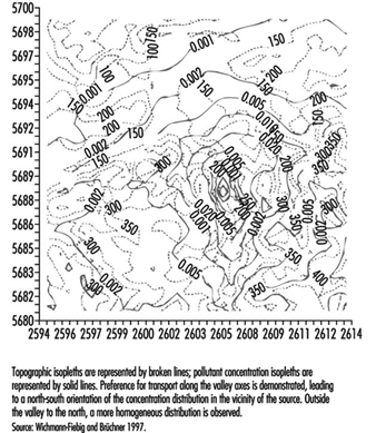
Figure 2. Topographic structure of a model region

Figure 2, figure 3 and figure 4 demonstrate how the transport and dispension of pollutants can be presented in relation to the influence of terrain and wind climatologies derived from consideration of surface and geostrophic wind frequencies.
Figure 3. Surface frequency distributions as determined from geostrophic frequency distribution
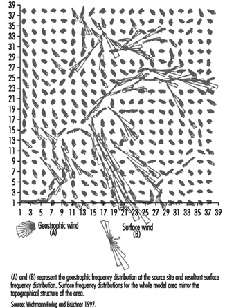
Figure 4. Annual mean pollutant concentrations for a hypothetical region calculated from the geostrophic frequency distribution for heterogeneous wind fields
Dispersion Modelling in Case of Low Sources
Considering air pollution caused by low sources (i.e., stack heights on the order of building height or emissions of road traffic) the influence of the surrounding buildings has to be considered. Road traffic emissions will be trapped to a certain amount in street canyons. Empirical formulations have been found to describe this (Yamartino and Wiegand 1986).
Pollutants emitted from a low stack situated on a building will be captured in the circulation on the lee side of the building. The extent of this lee circulation depends on the height and width of the building, as well as on wind speed. Therefore, simplified approaches to describe pollutant dispersion in such a case, based solely on the height of a building, are not generally valid. The vertical and horizontal extent of the lee circulation has been obtained from wind tunnel studies (Hosker 1985) and can be implemented in mass consistent diagnostic models. As soon as the flow field has been determined, it can be used to calculate the transport and turbulent mixing of the pollutant emitted. This can be done by Lagrangian or Eulerian dispersion modelling.
More detailed studies - concerning accidental releases, for instance - can be performed only by using non-hydrostatic flow and dispersion models instead of a diagnostic approach. As this, in general, demands high computer power, a worst case approach as described above is recommended in advance of a complete statistical modelling.
Air Quality Monitoring
Air quality monitoring means the systematic measurement of ambient air pollutants in order to be able to assess the exposure of vulnerable receptors (e.g., people, animals, plants and art works) on the basis of standards and guidelines derived from observed effects, and/or to establish the source of the air pollution (causal analysis).
Ambient air pollutant concentrations are influenced by the spatial or time variance of emissions of hazardous substances and the dynamics of their dispersion in the air. As a consequence, marked daily and annual variations of concentrations occur. It is practically impossible to determine in a unified way all these different variations of air quality (in statistical language, the population of air quality states). Thus, ambient air pollutant concentrations measurements always have the character of random spatial or time samples.
Measurement Planning
The first step in measurement planning is to formulate the purpose of the measurement as precisely as possible. Important questions and fields of operation for air quality monitoring include:
Area measurement:
- representative determination of exposure in one area (general air monitoring)
- representative measurement of pre-existing pollution in the area of a planned facility (permit, TA Luft (Technical instruction, air))
- smog warning (winter smog, high ozone concentrations)
- measurements in hot spots of air pollution to estimate maximum exposure of receptors (EU-NO2 guideline, measurements in street canyons, in accordance with the German Federal Immission Control Act)
- checking the results of pollution abatement measures and trends over time
- screening measurements
- scientific investigations - for example, the transport of air pollution, chemical conversions, calibrating dispersion calculations.
Facility measurement:
- measurements in response to complaints
- ascertaining sources of emissions, causal analysis
- measurements in cases of fires and accidental releases
- checking success of reduction measures
- monitoring factory fugitive emissions.
The goal of measurement planning is to use adequate measurement and assessment procedures to answer specific questions with sufficient certainty and at minimum possible expense.
An example of the parameters that should be used for measurement planning is presented in table 1, in relation to an assessment of air pollution in the area of a planned industrial facility. Recognizing that formal requirements vary by jurisdiction, it should be noted that specific reference here is made to German licensing procedures for industrial facilities.
Table 1. Parameters for measurement planning in measuring ambient air pollution concentrations (with example of application)
|
Parameter |
Example of application: Licensing procedure for |
|
Statement of the question |
Measurement of prior pollution in the licensing procedure; representative random probe measurement |
|
Area of measurement |
Circle around location with radius 30 times actual chimney height (simplified) |
|
Assessment standards (place and time dependent): characteristic values to be |
Threshold limits IW1 (arithmetic mean) and IW2 (98th percentile) of TA Luft (Technical instruction, air); calculation of I1 (arithmetic mean) and I2 (98th percentile) from measurements taken for 1 km2 (assessment surface) to be compared with IW1 and IW2 |
|
Ordering, choice and density |
Regular scan of 1km2, resulting in “random” choice of measurement sites |
|
Measurement time period |
1 year, at least 6 months |
|
Measurement height |
1.5 to 4 metres above ground |
|
Measurement frequency |
52 (104) measurements per assessment area for gaseous pollutants, depending on the height of the pollution |
|
Duration of each measurement |
1/2 hour for gaseous pollutants, 24 hours for suspended dust, 1 month for dust precipitation |
|
Measurement time |
Random choice |
|
Measured object |
Air pollution emitted from the planned facility |
|
Measurement procedure |
National standard measurement procedure (VDI guidelines) |
|
Necessary certainty of measurement results |
High |
|
Quality requirements, quality control, calibration, maintenance |
VDI guidelines |
|
Recording of measurement data, validation, archiving, assessment |
Calculation of quantity of data I1V and I2V for every assessment area |
|
Costs |
Depend on measurement area and objectives |
The example in table 1 shows the case of a measurement network that is supposed to monitor the air quality in a specific area as representatively as possible, to compare with designated air quality limits. The idea behind this approach is that a random choice of measurement sites is made in order to cover equally locations in an area with varying air quality (e.g., living areas, streets, industrial zones, parks, city centres, suburbs). This approach may be very costly in large areas due to the number of measurement sites necessary.
Another conception for a measurement network therefore starts with measurement sites that are representatively selected. If measurements of differing air quality are conducted in the most important locations, and the length of time that the protected objects remain in these “microenvironments” is known, then the exposure can be determined. This approach can be extended to other microenvironments (e.g., interior rooms, cars) in order to estimate the total exposure. Diffusion modelling or screening measurements can help in choosing the right measurement sites.
A third approach is to measure at the points of presumed highest exposure (e.g., for NO2 and benzene in street canyons). If assessment standards are met at this site, there is sufficient probability that this will also be the case for all other sites. This approach, by focusing on critical points, requires relatively few measurement sites, but these must be chosen with particular care. This particular method risks overestimating real exposure.
The parameters of measurement time period, assessment of the measurement data and measurement frequency are essentially given in the definition of the assessment standards (limits) and the desired level of certainty of the results. Threshold limits and the peripheral conditions to be considered in measurement planning are related. By using continuous measurement procedures, a resolution that is temporally almost seamless can be achieved. But this is necessary only in monitoring peak values and/or for smog warnings; for monitoring annual mean values, for example, discontinuous measurements are adequate.
The following section is dedicated to describing the capabilities of measurement procedures and quality control as a further parameter important to measurement planning.
Quality Assurance
Measurements of ambient air pollutant concentrations can be costly to conduct, and results can affect significant decisions with serious economic or ecological implications. Therefore, quality assurance measures are an integral part of the measurement process. Two areas should be distinguished here.
Procedure-oriented measures
Every complete measurement procedure consists of several steps: sampling, sample preparation and clean-up; separation, detection (final analytical step); and data collection and assessment. In some cases, especially with continuous measurement of inorganic gases, some steps of the procedure can be left out (e.g., separation). Comprehensive adherence to procedures should be strived for in conducting measurements. Procedures that are standardized and thus comprehensively documented should be followed, in the form of DIN/ISO standards, CEN standards or VDI guidelines.
User-oriented measures
Using standardized and proven equipment and procedures for ambient air pollutant concentration measurement cannot alone ensure acceptable quality if the user does not employ adequate methods of quality control. The standards series DIN/EN/ISO 9000 (Quality Management and Quality Assurance Standards), EN 45000 (which defines the requirements for testing laboratories) and ISO Guide 25 (General Requirements for the Competence of Calibration and Testing Laboratories) are important for user-oriented measures to ensure quality.
Important aspects of user quality control measures include:
- acceptance and practice of the content of the measures in the sense of good laboratory practice (GLP)
- correct maintenance of measurement equipment, qualified measures to eliminate disruptions and ensure repairs
- carrying out calibrations and regular checking to ensure proper functioning
- carrying out interlaboratory testing.
Measurement Procedures
Measurement procedures for inorganic gases
A wealth of measurement procedures exists for the broad range of inorganic gases. We will differentiate between manual and automatic methods.
Manual procedures
In the case of manual measurement procedures for inorganic gases, the substance to be measured is normally adsorbed during the sampling in a solution or solid material. In most cases a photometric determination is made after an appropriate colour reaction. Several manual measurement procedures have special significance as reference procedures. Because of the relatively high personnel cost, these manual procedures are conducted only rarely for field measurements today, when alternative automatic procedures are available. The most important procedures are briefly sketched in table 2.
Table 2. Manual measurement procedures for inorganic gases
|
Material |
Procedure |
Execution |
Comments |
|
SO2 |
TCM procedure |
Absorption in tetrachloromercurate solution (wash bottle); reaction with formaldehyde and pararosaniline to red-violet sulphonic acid; photometric determination |
EU-reference measurement procedure; |
|
SO2 |
Silica gel procedure |
Removal of interfering substances by concentrated H3PO4; adsorption on silica gel; thermal desorption in H2-stream and reduction to H2S; reaction to molybdenum-blue; photometric determination |
DL = 0.3 µg SO2; |
|
NO2 |
Saltzman procedure |
Absorption in reaction solution while forming a red azo dye (wash bottle); photometric determination |
Calibration with sodium nitrite; |
|
O3 |
Potassium iodide |
Formation of iodine from aqueous potassium iodide solution (wash bottle); photometric determination |
DL = 20 µg/m3; |
|
F– |
Silver bead procedure; |
Sampling with dust preseparator; enrichment of F– on sodium carbonate-coated silver beads; elution and measurement with ion-sensitive lanthanum fluoride-electrode chain |
Inclusion of an undetermined portion of particulate fluoride immissions |
|
F– |
Silver bead procedure; |
Sampling with heated membrane filter; enrichment of F– on sodium carbonate-coated silver beads; determination by electrochemical (variant 1) or photometric (alizarin-complexone) procedure |
Danger of lower findings due to partial sorption of gaseous fluoride immissions on membrane filter; |
|
Cl– |
Mercury rhodanide |
Absorption in 0.1 N sodium hydroxide solution (wash bottle); reaction with mercury rhodanide and Fe(III) ions to iron thiocyanato complex; photometric determination |
DL = 9 µg/m3 |
|
Cl2 |
Methyl-orange procedure |
Bleaching reaction with methyl-orange solution (wash bottle); photometric determination |
DL = 0.015 mg/m3 |
|
NH3 |
Indophenol procedure |
Absorption in dilute H2SO4 (Impinger/wash bottle); conversion with phenol and hypochlorite to indophenol dye; photometric determination |
DL = 3 µg/m3 (impinger); partial |
|
NH3 |
Nessler procedure |
Absorption in dilute H2SO4 (Impinger/wash bottle); distillation and reaction with Nessler’s reagent, photometric determination |
DL = 2.5 µg/m3 (impinger); partial |
|
H2S |
Molybdenum-blue |
Absorption as silver sulphide on glass beads treated with silver sulphate and potassium hydrogen sulphate (sorption tube); released as hydrogen sulphide and conversion to molybdenum blue; photometric determination |
DL = 0.4 µg/m3 |
|
H2S |
Methylene blue procedure |
Absorption in cadmium hydroxide suspension while forming CdS; conversion to methylene blue; photometric determination |
DL = 0.3 µg/m3 |
DL = detection limit; s = standard deviation; rel. s = relative s.
A special sampling variant, used primarily in connection with manual measurement procedures, is the diffusion separation tube (denuder). The denuder technique is aimed at separating the gas and particle phases by using their different diffusion rates. Thus, it is often used on difficult separation problems (e.g., ammonia and ammonium compounds; nitrogen oxides, nitric acid and nitrates; sulphur oxides, sulphuric acid and sulphates or hydrogen halides/halides). In the classic denuder technique, the test air is sucked through a glass tube with a special coating, depending on the material(s) to be collected. The denuder technique has been further developed in many variations and also partially automated. It has greatly expanded the possibilities of differentiated sampling, but, depending on the variant, it can be very laborious, and proper utilization requires a great deal of experience.
Automated procedures
There are numerous different continuous measuring monitors on the market for sulphur dioxide, nitrogen oxides, carbon monoxide and ozone. For the most part they are used particularly in measurement networks. The most important features of the individual methods are collected in table 3.
Table 3. Automated measurement procedures for inorganic gases
|
Material |
Measuring principle |
Comments |
|
SO2 |
Conductometry reaction of SO2 with H2O2 in dilute H2SO4; measurement of increased conductivity |
Exclusion of interferences with selective filter (KHSO4/AgNO3) |
|
SO2 |
UV fluorescence; excitationof SO2 molecules with UV radiation (190–230 nm); measurement of fluorescence radiation |
Interferences, e.g., by hydrocarbons, |
|
NO/NO2 |
Chemiluminescence; reaction of NO with O3 to NO2; detection of chemiluminescence radiation with photomultiplier |
NO2 only indirectly measurable; use of converters for reduction of NO2 to NO; measurement of NO and NOx |
|
CO |
Non-dispersive infrared absorption; |
Reference: (a) cell with N2; (b) ambient air after removal of CO; (c) optical removal of CO absorption (gas filter correlation) |
|
O3 |
UV absorption; low-pressure Hg lamp as radiation source (253.7 nm); registration of UV absorption in accordance with Lambert-Beer’s law; detector: vacuum photodiode, photosensitive valve |
Reference: ambient air after removal of ozone (e.g., Cu/MnO2) |
|
O3 |
Chemiluminescence; reaction of O3 with ethene to formaldehyde; detection of chemiluminescence radiation with |
Good selectivity; ethylene necessary as reagent gas |
It should be emphasized here that all automatic measurement procedures based on chemical-physical principles must be calibrated using (manual) reference procedures. Since automatic equipment in measurement networks often runs for extended periods of time (e.g., several weeks) without direct human supervision, it is indispensable that their correct functioning is regularly and automatically checked. This generally is done using zero and test gases that can be produced by several methods (preparation of ambient air; pressurized gas cylinders; permeation; diffusion; static and dynamic dilution).
Measurement procedures for dust-forming air pollutants and its composition
Among particulate air pollutants, dustfall and suspended particulate matter (SPM) are differentiated. Dustfall consists of larger particles, which sink to the ground because of their size and thickness. SPM includes the particle fraction that is dispersed in the atmosphere in a quasi-stable and quasi-homogenous manner and therefore remains suspended for a certain time.
Measurement of suspended particulate matter and metallic compounds in SPM
As is the case with measurements of gaseous air pollutants, continuous and discontinuous measurement procedures for SPM can be differentiated. As a rule, SPM is first separated on glass fibre or membrane filters. It follows a gravimetric or radiometric determination. Depending on the sampling, a distinction can be made between a procedure to measure the total SPM without fractionation according to the size of the particles and a fractionation procedure to measure the fine dust.
The advantages and disadvantages of fractionated suspended dust measurements are disputed internationally. In Germany, for example, all threshold limits and assessment standards are based on total suspended particulates. This means that, for the most part, only total SPM measurements are performed. In the United States, on the contrary, the so-called PM-10 procedure (particulate matter £ 10μm) is very common. In this procedure, only particles with an aerodynamic diameter up to 10 μm are included (50 per cent inclusion portion), which are inhalable and can enter the lungs. The plan is to introduce the PM-10 procedure into the European Union as a reference procedure. The cost for fractionated SPM measurements is considerably higher than for measuring total suspended dust, because the measuring devices must be fitted with special, expensively constructed sampling heads that require costly maintenance. Table 4 contains details on the most important SPM measurement procedures.
Table 4. Measurement procedures for suspended particulate matter (SPM)
|
Procedure |
Measuring principle |
Comments |
|
Small filter device |
Non-fractionated sampling; air flow rate 2.7–2.8 m3/h; filter diameter 50 mm; gravimetric analysis |
Easy handling; control clock; |
|
LIB device |
Non-fractionated sampling; air flow rate 15-16 m3/h; filter diameter 120 mm; gravimetric analysis |
Separation of large dust |
|
High-Volume-Sampler |
Inclusion of particles up to approx. 30 µm diameter; air flow rate approx. 100 m3/h; filter diameter 257 mm; gravimetric analysis |
Separation of large dust |
|
FH 62 I |
Continuous, radiometric dust measuring device; non-fractionating sampling; air flow rate 1 or 3 m3/h; registration of dust mass separated on a filter band by measuring attenuation of β-radiation (krypton 85) in passage through exposed filter (ionization chamber) |
Gravimetric calibration by dusting of single filters; device also operable with PM-10 preseparator |
|
BETA dust meter F 703 |
Continuous, radiometric dust measuring device; non-fractionated sampling; air flow rate 3 m3/h; registration of dust mass separated on a filter band by measuring attenuation of β-radiation (carbon 14) in passage through exposed filter (Geiger Müller counter tube) |
Gravimetric calibration by dusting of single filters; device also operable with PM-10 preseparator |
|
TEOM 1400 |
Continuous dust measuring device; non-fractionated sampling; air flow rate 1 m3/h; dust collected on a filter, which is part of a self-resonating, vibrating system, in side stream (3 l/min); registration of the frequency lowering by increased dust load on the filter |
Relationship between frequency
|
Recently, automatic filter changers have also been developed that hold a larger number of filters and supply them to the sampler, one after another, at timed intervals. The exposed filters are stored in a magazine. The detection limits for filter procedures lie between 5 and 10 μg/m3 of dust, as a rule.
Finally, the black smoke procedure for SPM measurements has to be mentioned. Coming from Britain, it has been incorporated into EU guidelines for SO2 and suspended dust. In this procedure, the blackening of the coated filter is measured with a reflex photometer after the sampling. The black smoke values that are thus photometrically obtained are converted into gravimetric units (μg/m3) with the help of a calibration curve. Since this calibration function depends to a high degree on the composition of the dust, especially its soot content, the conversion into gravimetric units is problematic.
Today, metal compounds are often routinely determined in suspended dust immission samples. In general, the collection of the suspended dust on filters is followed by a chemical dissolution of the separated dusts, since the most common final analytical steps presuppose converting the metallic and metalloid compounds in an aqueous solution. In practice, the most important methods by far are atom absorption spectroscopy (AAS) and spectroscopy with plasma excitation (ICP-OES). Other procedures for determining metallic compounds in suspended dust are x-ray fluorescence analysis, polarography and neutron activation analysis. Although metallic compounds have been measured for more than a decade now as a component of SPM in outside air at certain measurement sites, important unanswered questions remain. Thus the conventional sampling by separating the suspended dust on filters assumes that the separation of the heavy metal compounds on the filter is complete. However, earlier indications have been found in the literature questioning this. The results are very heterogeneous.
A further problem lies in the fact that different compound forms, or single compounds of the respective elements, cannot be distinguished in the analysis of metallic compounds in suspended dust using the conventional measurement procedures. While in many cases adequate total determinations can be made, a more thorough differentiation would be desirable with certain especially carcinogenic metals (As, Cd, Cr, Ni, Co, Be). There are often big differences in the carcinogenic effects of elements and their individual compounds (e.g., chromium compounds in oxidation levels III and VI - only those in level VI are carcinogenic). In such cases a specific measurement of the individual compounds (species analysis) would be desirable. Despite the significance of this problem, only first attempts at species analysis are being made in measurement technique.
Measurement of dustfall and metallic compounds in dustfall
Two fundamentally different methods are used to collect dustfall:
- sampling in collecting vessels
- sampling on adhesive surfaces.
A popular procedure for measuring dustfall (deposited dust) is the so-called Bergerhoff procedure. In this procedure the entire atmospheric precipitation (dry and wet depositions) is collected over 30± 2 days in vessels about 1.5 to 2.0 metres above the ground (bulk deposition). Then the collecting vessels are taken to the lab and prepared (filtered, water evaporated, dried, weighed). The result is calculated on the basis of the surface area of the collecting vessel and exposure time in grams per square meter and day (g/m2d). The relative detection limit is 0.035 g/m2d.
Additional procedures for collecting dustfall include the Liesegang-Löbner device and methods which collect the deposited dust on adhesive foils.
All measurement results for dustfall are relative values that depend on the apparatus used, as the dust separation is influenced by the flow conditions at the device and other parameters. The differences in the measurement values obtained with the different procedures can reach 50 per cent.
Also important is the composition of the deposited dust, such as the content of lead, cadmium and other metallic compounds. The analytical procedures used for this are basically the same as those used for suspended dust.
Measuring special materials in dust form
Special materials in dust form include asbestos and soot. Collecting fibres as air pollutants is important since asbestos has been classified as a confirmed carcinogenic material. Fibres with a diameter of D ≤ 3μm and a length of L ≥ 5μm, where L:D ≥ 3, are considered carcinogenic. Measurement procedures for fibrous materials consist of counting, under the microscope, fibres that have been separated on filters. Only electron microscopic procedures can be considered for outside air measurements. The fibres are separated on gold-coated porous filters. Prior to assessment in an electron scan microscope, the sample is freed of organic substances through plasma incineration right on the filter. The fibres are counted on part of the filter surface, randomly chosen and classified by geometry and type of fibre. With the help of energy dispersive x-ray analysis (EDXA), asbestos fibres, calcium sulphate fibres and other inorganic fibres can be differentiated on the basis of elemental composition. The entire procedure is extremely expensive and requires the greatest care to achieve reliable results.
Soot in the form of particles emitted by diesel motors has become relevant since diesel soot was also classified as carcinogenic. Because of its changing and complex composition and because of the fact that various constituents are also emitted from other sources, there is no measurement procedure specific to diesel soot. Nevertheless, in order to say something concrete about the concentrations in ambient air, soot is conventionally defined as elemental carbon, as a part of total carbon. It is measured after sampling and an extraction step and/or thermal desorption. Determination of the carbon content ensues through burning in an oxygen stream and coulometric titration or non-dispersive IR detection of the carbon dioxide formed in the process.
The so-called aethalometer and the photoelectric aerosol sensor are also used for measuring soot, in principle.
Measuring Wet Depositions
Together with dry deposition, wet deposition in rain, snow, fog and dew constitute the most important means by which harmful materials enter the ground, water or plant surfaces from the air.
In order to clearly distinguish the wet deposition in rain and snow (fog and dew present special problems) from the measurement of total deposition (bulk deposition, see section “Measurement of dustfall and metallic compounds” above) and dry deposition, rain catchers, whose collection opening is covered when there is no rain (wet-only sampler), are used for sampling. With rain sensors, which mostly work on the principle of conductivity changes, the cover is opened when it starts to rain and closed again when the rain stops.
The samples are transferred through a funnel (open area approx. 500 cm2 and more) into a darkened and if possible insulated collection container (of glass or polyethylene for inorganic components only).
In general, analysing the collected water for inorganic components can be done without sample preparation. The water should be centrifuged or filtered if it is visibly cloudy. The conductivity, pH value and important anions (NO3 – , SO4 2– , Cl–) and cations (Ca2+, K+, Mg2+, Na+, NH4 + and so on) are routinely measured. Unstable trace compounds and intermediate states like H2O2 or HSO3 – are also measured for research purposes.
For analysis, procedures are used that are generally available for aqueous solutions such as conductometry for conductivity, electrodes for pH values, atom adsorption spectroscopy for cations (see section “Measuring special materials in dust form”, above) and, increasingly, ion exchange chromatography with conductivity detection for anions.
Organic compounds are extracted from rain water with, for example, dichloromethane, or blown out with argon and adsorbed with Tenax tubes (only highly volatile materials). The materials are then subjected to a gas chromatographic analysis (see “Measurement procedures for organic air pollutants”, below).
Dry deposition correlates directly with ambient air concentrations. The concentration differences of airborne harmful materials in rain, however, are relatively small, so that for measuring wet deposition, wide-mesh measuring networks are adequate. Examples include the European EMEP measurement network, in which the entry of sulphate and nitrate ions, certain cations and precipitation pH values are collected in approximately 90 stations. There are also extensive measurement networks in North America.
Optical Long-Distance Measurement Procedures
Whereas the procedures described up to now catch air pollution at one point, optical long-distance measuring procedures measure in an integrated manner over light paths of several kilometres or they determine the spatial distribution. They use the absorption characteristics of gases in the atmosphere in the UV, visible or IR spectral range and are based on the Lambert-Beer law, according to which the product of light path and concentration are proportional to the measured extinction. If the sender and receiver of the measuring installation change the wavelength, several components can be measured in parallel or sequentially with one device.
In practice, the measurement systems identified in table 5 play the biggest role.
Table 5. Long-distance measurement procedures
|
Procedure |
Application |
Advantages, disadvantages |
|
Fourier |
IR range (approx. 700–3,000 cm–1), several hundred metres light path. |
+ Multi-component system |
|
Differential |
Light path to several km; measures SO2, NO2, benzene, HNO3; monitors linear and surface sources, used in measuring networks |
+ Easy to handle |
|
Long-distance |
Research area, in low-pressure cuvettes for OH- |
+ High sensitivity (to ppt) |
|
Differential |
Monitors surface sources, large surface immission measurements |
+ Measurements of spatial |
LIDAR = Light detection and ranging; DIAL = differential absorption LIDAR.
Measurement Procedures for Organic Air Pollutants
The measurement of air pollution containing organic components is complicated primarily by the range of materials in this class of compounds. Several hundred individual components with very different toxicological, chemical and physical characteristics are covered under the general title “organic air pollutants” in the emissions registers and air quality plans of congested areas.
Especially due to the great differences in potential impact, collecting relevant individual components has more and more taken the place of previously used summation procedures (e.g., Flame Ionization Detector, total carbon procedure), the results of which cannot be assessed toxicologically. The FID method, however, has retained a certain significance in connection with a short separation column to separate out methane, which is photochemically not very reactive, and for collecting the precursor volatile organic compounds (VOC) for the formation of photo-oxidants.
The frequent necessity of separating the complex mixtures of the organic compounds into relevant individual components makes measuring it virtually an exercise in applied chromatography. Chromatographic procedures are the methods of choice when the organic compounds are sufficiently stable, thermally and chemically. For organic materials with reactive functional groups, separate procedures that use the functional groups’ physical characteristics or chemical reactions for detection continue to hold their ground.
Examples include using amines to convert aldehydes to hydrazones, with subsequent photometric measurement; derivatization with 2,4-dinitrophenylhydrazine and separation of the 2,4-hydrazone that is formed; or forming azo-dyes with p-nitroaniline for detecting phenols and cresols.
Among chromatographic procedures, gas chromatography (GC) and high-pressure liquid chromatography (HPLC) are most frequently employed for separating the often complex mixtures. For gas chromatography, separation columns with very narrow diameters (approx. 0.2 to 0.3 mm, and approx. 30 to 100 m long), so-called high-resolution capillary columns (HRGC), are almost exclusively utilized today. A series of detectors are available for finding the individual components after the separation column, such as the above-mentioned FID, the ECD (electron capture detector, specifically for electrophilic substitutes such as halogen), the PID (photo-ionization detector, which is especially sensitive to aromatic hydrocarbons and other p-electron systems), and the NPD (thermo-ionic detector specifically for nitrogen and phosphorus compounds). The HPLC uses special through-flow detectors which, for example, are designed as the through-flow cuvette of a UV spectrometer.
Especially effective, but also especially expensive, is the use of a mass spectrometer as a detector. Really certain identification, especially with unknown mixtures of compounds, is often possible only through the mass spectrum of the organic compound. The qualitative information of the so-called retention time (time the material remains in the column) that is contained in the chromatogram with conventional detectors is supplemented with the specific detection of the individual components by mass fragmentograms with high detection sensitivity.
Sampling must be considered before the actual analysis. The choice of sampling method is determined primarily by volatility, but also by expected concentration range, polarity and chemical stability. Furthermore, with non-volatile compounds, a choice must be made between concentration and deposition measurements.
Table 6 provides an overview of common procedures in air monitoring for active enrichment and chromatographic analysis of organic compounds, with examples of applications.
Table 6. Overview of common chromatographic air quality measurement procedures of organic compounds (with examples of applications)
|
Material group |
Concentration |
Sampling, preparation |
Final analytical step |
|
Hydrocarbons C1–C9 |
μg/m3 |
Gas mice (rapid sampling), gas-tight syringe, cold trapping in front of capillary column (focusing), thermal desorption |
GC/FID |
|
Low-boiling hydrocarbons, highly |
ng/m3–μg/m3 |
Evacuated, passivated high-grade steel cylinder (also for clean air measurements) |
GC/FID/ECD/PID |
|
Organic compounds in boiling point |
μg/m3 |
Adsorption on activated carbon, (a) desorption with CS2 (b) desorption with solvents (c) headspace analysis |
Capillary |
|
Organic compounds in boiling point |
ng/m3–μg/m3 |
Adsorption on organic polymers (e.g., Tenax) or molecular carbon sieve (carbopack), thermal desorption with cold trapping in front of capillary column (focusing) or solvent extraction |
Capillary |
|
Modification for low-boiling |
ng/m3–μg/m3 |
Adsorption on cooled polymers (e.g. thermogradient tube), cooled to –120 ºC, use of carbopack |
Capillary |
|
High boiling organic compounds |
fg/m3–ng/m3 |
Sampling on filters (e.g., small filter device or high volume sampler) with subsequent polyurethane cartridges for gaseous portion, solvent desorption of filter and polyurethane, various purification and preparatory steps, for PAH also sublimation |
Capillary |
|
High boiling organic compounds, |
fg/m3–ng/m3 |
Adsorption on organic polymers (e.g., polyurethane foam cylinder) with prior filters (e.g., glass fibre) or inorg. adsorp. (e.g., silica gel), extraction with solvents, various purification and preparatory steps, (including multicolumn chromatography), derivatizing for chlorophenols |
HRGC/ECD |
|
High boiling organic compounds |
ng/m3 |
Separation of aerosols on glass fibre filters (e.g., high or low volume sampler) or dust collection on standardized surfaces, extraction with solvents (for deposition also of remaining filtered water), various purification and preparation steps |
HRGC/MS |
GC = gas chromatography; GCMS = GC/mass spectroscopy; FID = flame ionization detector; HRGC/ECD = high resolution GC/ECD; ECD = electron capture detector; HPLC = high performance liquid chromatography. PID = photo-ionization detector.
Deposition measurements of organic compounds with low volatility (e.g., dibenzodioxins and dibenzofurans (PCDD/PCDF), polycyclic aromatic hydrocarbons (PAH)) are gaining in importance from the perspective of environmental impact. Since food is the main source of human intake, airborne material transferred onto food plants is of great significance. There is, however, evidence that material transfer by way of particulate deposition is less important than dry deposition of quasi-gaseous compounds.
For measuring total deposition, standardized devices for dust precipitation are used (e.g., Bergerhoff procedure), which have been slightly modified by darkening as a protection against the entry of strong light. Important technical measurement problems, such as the resuspension of already separated particles, evaporation or possible photolytic decomposition, are now being systematically researched in order to improve the less-than-optimal sampling procedures for organic compounds.
Olfactometric Investigations
Olfactometric immission investigations are used in monitoring to quantify odour complaints and to determine baseline pollution in licensing procedures. They serve primarily to assess whether existing or anticipated odours should be classified as significant.
In principle, three methodological approaches can be differentiated:
- measurement of the emission concentration (number of odour units) with an olfactometer and subsequent dispersion modelling
- measurement of individual components (e.g., NH3) or mixtures of compounds (e.g., gas chromatography of gases from landfills), if these adequately characterize the odour
- odour determinations by means of inspections.
The first possibility combines emission measurement with modelling and, strictly speaking, cannot be classified under the term air quality monitoring. In the third method, the human nose is used as the detector with significantly reduced precision as compared to physical-chemical methods.
Details of inspections, measurement plans and assessing the results are contained, for example, in the environmental protection regulations of some German states.
Screening Measurement Procedures
Simplified measurement procedures are sometimes used for preparatory studies (screening). Examples include passive samplers, test tubes and biological procedures. With passive (diffusive) samplers, the material to be tested is collected with freely flowing processes such as diffusion, permeation or adsorption in simple forms of collectors (tubes, plaques) and enriched in impregnated filters, meshes or other adsorption media. So-called active sampling (sucking the sample air through a pump) thus does not occur. The enriched quantity of material, analytically determined according to definite exposure time, is converted into concentration units on the basis of physical laws (e.g., of diffusion) with the help of collection time and the collector’s geometric parameters. The methodology stems from the field of occupational health (personal sampling) and indoor air measurement, but it is increasingly being used for ambient air pollutant concentration measurements. An overview can be found in Brown 1993.
Detector tubes are often used for sampling and quick preparatory analysis of gases. A certain test air volume is sucked through a glass tube that is filled with an adsorptive reagent that corresponds with the test objective. The contents of the tube change colour depending on the concentration of the material to be determined that is present in the test air. Small testing tubes are often used in the field of workplace monitoring or as a quick procedure in cases of accidents, such as fires. They are not used for routine ambient air pollutant concentration measurements due to the generally too high detection limits and too limited selectivity. Detector testing tubes are available for numerous materials in various concentration ranges.
Among the biological procedures, two methods have become accepted in routine monitoring. With the standardized lichen exposure procedure, the mortality rate of the lichen is determined over the exposure time of 300 days. In another procedure, French pasture grass is exposed for 14±1 days. Then the amount of growth is determined. Both procedures serve as summary determinations of air pollutant concentration effects.
Air Quality Monitoring Networks
Around the world, the most varied types of air quality networks are utilized. A distinction should be drawn between measurement networks, consisting of automatic, computer-controlled measuring stations (measurement containers), and virtual measurement networks, which only define the measurement locations for various types of air pollutant concentration measurements in the form of a preset grid. Tasks and conceptions of measurement networks were discussed above.
Continuous monitoring networks
Continuously operating measurement networks are based on automatic measuring stations, and serve primarily for air quality monitoring of urban areas. Measured are air pollutants such as sulphur dioxide (SO2), dust, nitrogen monoxide (NO), nitrogen dioxide (NO2), carbon monoxide (CO), ozone (O3), and to an extent also the sum of the hydrocarbons (free methane, CnHm) or individual organic components (e.g., benzene, toluene, xylenes). In addition, depending on need, meteorological parameters such as wind direction, wind speed, air temperature, relative humidity, precipitation, global radiation or radiation balance are included.
The measuring equipment operated in measurement stations generally consists of an analyser, a calibration unit, and control and steering electronics, which monitors the whole measuring equipment and contains a standardized interface for data collection. In addition to the measurement values, the measuring equipment supplies so-called status signals on errors and the operating status. The calibration of the devices is automatically checked by computer at regular intervals.
As a rule, the measurement stations are connected with fixed data lines, dial connections or other data transfer systems to a computer (process computer, workstation or PC, depending on the scope of the system) in which the measurement results are entered, processed and displayed. The measurement network computers and, if necessary, specially trained personnel monitor continuously whether various threshold limits are exceeded. In this manner critical air quality situations can be recognized at any time. This is very important, especially for monitoring critical smog situations in winter and summer (photo-oxidants) and for current public information.
Measurement networks for random sample measurements
Beyond the telemetric measurement network, other measuring systems for monitoring air quality are used to varying extents. Examples include (occasionally partially automated) measurement networks to determine:
- dust deposition and its components
- suspended dust (SPM) and its components
- hydrocarbons and chlorinated hydrocarbons
- low volatile organic materials (dioxins, furans, polychlorinated biphenyls).
A series of substances measured in this manner have been classified as carcinogens, such as cadmium compounds, PAHs or benzene. Monitoring them is therefore particularly important.
To provide an example of a comprehensive programme, table 7 summarizes the air quality monitoring that is systematically conducted in North Rhine-Westphalia, which with 18 million inhabitants is the most populous state in Germany.
Table 7. Systematic air quality monitoring in North-Rhine-Westphalia (Germany)
|
Continuous measuring |
Partially automated |
Discontinuous measuring |
|
Sulphur dioxide |
SPM composition: |
Benzene and other |
Air Pollution Control
Management of Air Pollution
The objective of a manager of an air pollution control system is to ensure that excessive concentrations of air pollutants do not reach a susceptible target. Targets could include people, plants, animals and materials. In all cases we should be concerned with the most sensitive of each of these groups. Air pollutants could include gases, vapours, aerosols and, in some cases, biohazardous materials. A well designed system will prevent a target from receiving a harmful concentration of a pollutant.
Most air pollution control systems involve a combination of several control techniques, usually a combination of technological controls and administrative controls, and in larger or more complex sources there may be more than one type of technological control.
Ideally, the selection of the appropriate controls will be made in the context of the problem to be solved.
- What is emitted, in what concentration?
- What are the targets? What is the most susceptible target?
- What are acceptable short-term exposure levels?
- What are acceptable long-term exposure levels?
- What combination of controls must be selected to ensure that the short-term and long-term exposure levels are not exceeded?
Table 1 describes the steps in this process.
Table 1. Steps in selecting pollution controls
|
Step 1: |
The first part is to determine what will be released from the stack. |
|
Step 2: |
All susceptible targets should be identified. This includes people, animals, plants and materials. In each case, the most susceptible member of each group must be identified. For example, asthmatics near a plant that emits isocyanates. |
|
Step 3: |
An acceptable level of exposure for the most sensitive target group must |
|
Step 4: |
Step 1 identifies the emissions, and Step 3 determines the acceptable |
* When setting exposure levels in Step 3, it must be remembered that these exposures are total exposures, not just those from the plant. Once the acceptable level has been established, background levels, and contributions from other plants just be subtracted to determine the maximum amount that the plant can emit without exceeding the acceptable exposure level. If this is not done, and three plants are allowed to emit at the maximum amount, the target groups will be exposed to three times the acceptable level.
** Some materials such as carcinogens do not have a threshold below which no harmful effects will occur. Therefore, as long as some of the material is allowed to escape to the environment, there will be some risk to the target populations. In this case a no effect level cannot be set (other than zero). Instead, an acceptable level of risk must be established. Usually this is set in the range of 1 adverse outcome in 100,000 to 1,000,000 exposed persons.
Some jurisdictions have done some of the work by setting standards based on the maximum concentration of a contaminant that a susceptible target can receive. With this type of standard, the manager does not have to carry out Steps 2 and 3, since the regulating agency has already done this. Under this system, the manager must establish only the uncontrolled emission standards for each pollutant (Step 1), and then determine what controls are necessary to meet the standard (Step 4).
By having air quality standards, regulators can measure individual exposures and thus determine whether anyone is exposed to potentially harmful levels. It is assumed that the standards set under these conditions are low enough to protect the most susceptible target group. This is not always a safe assumption. As shown in table 2, there can be a wide variation in common air quality standards. Air quality standards for sulphur dioxide range from 30 to 140 μg/m3. For less commonly regulated materials this variation can be even larger (1.2 to 1,718 μg/m3), as shown in table 3 for benzene. This is not surprising given that economics can play as large a role in standard setting as does toxicology. If a standard is not set low enough to protect susceptible populations, no one is well served. Exposed populations have a feeling of false confidence, and can unknowingly be put at risk. The emitter may at first feel that they have benefited from a lenient standard, but if effects in the community require the company to redesign their controls, or install new controls, costs could be higher than doing it correctly the first time.
Table 2. Range of air quality standards for a commonly controlled air contaminant (sulphur dioxide)
|
Countries and territories |
Long-term sulphur dioxide |
|
Australia |
50 |
|
Canada |
30 |
|
Finland |
40 |
|
Germany |
140 |
|
Hungary |
70 |
|
Taiwan |
133 |
Table 3. Range of air quality standards for a less commonly controlled air contaminant (benzene)
|
City/State |
24-hour air quality standard for |
|
Connecticut |
53.4 |
|
Massachusetts |
1.2 |
|
Michigan |
2.4 |
|
North Carolina |
2.1 |
|
Nevada |
254 |
|
New York |
1,718 |
|
Philadelphia |
1,327 |
|
Virginia |
300 |
The levels were standardized to an averaging time of 24 hours to assist in the comparisons.
(Adapted from Calabrese and Kenyon 1991.)
Sometimes this stepwise approach to selecting air pollution controls is short circuited, and the regulators and designers go directly to a “universal solution”. One such method is best available control technology (BACT). It is assumed that by using the best combination of scrubbers, filters and good work practices on an emission source, a level of emissions low enough to protect the most susceptible target group would be achieved. Frequently, the resulting emission level will be below the minimum required to protect the most susceptible targets. This way all unnecessary exposures should be eliminated. Examples of BACT are shown in table 4.
Table 4. Selected examples of best available control technology (BACT) showing the control method used and estimated efficiency
|
Process |
Pollutant |
Control method |
Estimated efficiency |
|
Soil remediation |
Hydrocarbons |
Thermal oxidizer |
99 |
|
Kraft pulp mill |
Particulates |
Electrostatic |
99.68 |
|
Production of fumed |
Carbon monoxide |
Good practice |
50 |
|
Automobile painting |
Hydrocarbons |
Oven afterburner |
90 |
|
Electric arc furnace |
Particulates |
Baghouse |
100 |
|
Petroleum refinery, |
Respirable particulates |
Cyclone + Venturi |
93 |
|
Medical incinerator |
Hydrogen chloride |
Wet scrubber + dry |
97.5 |
|
Coal-fired boiler |
Sulphur dioxide |
Spray dryer + |
90 |
|
Waste disposal by |
Particulates |
Cyclone + condenser |
95 |
|
Asphalt plant |
Hydrocarbons |
Thermal oxidizer |
99 |
BACT by itself does not ensure adequate control levels. Although this is the best control system based on gas cleaning controls and good operating practices, BACT may not be good enough if the source is a large plant, or if it is located next to a sensitive target. Best available control technology should be tested to ensure that it is indeed good enough. The resulting emission standards should be checked to determine whether or not they may still be harmful even with the best gas cleaning controls. If emission standards are still harmful, other basic controls, such as selecting safer processes or materials, or relocating in a less sensitive area, may have to be considered.
Another “universal solution” that bypasses some of the steps is source performance standards. Many jurisdictions establish emission standards that cannot be exceeded. Emission standards are based on emissions at the source. Usually this works well, but like BACT they can be unreliable. The levels should be low enough to maintain the maximum emissions low enough to protect susceptible target populations from typical emissions. However, as with best available control technology, this may not be good enough to protect everyone where there are large emission sources or nearby susceptible populations. If this is the case, other procedures must be used to ensure the safety of all target groups.
Both BACT and emission standards have a basic fault. They assume that if certain criteria are met at the plant, the target groups will be automatically protected. This is not necessarily so, but once such a system is passed into law, effects on the target become secondary to compliance with the law.
BACT and source emission standards or design criteria should be used as minimum criteria for controls. If BACT or emission criteria will protect the susceptible targets, then they can be used as intended, otherwise other administrative controls must be used.
Control Measures
Controls can be divided into two basic types of controls - technological and administrative. Technological controls are defined here as the hardware put on an emission source to reduce contaminants in the gas stream to a level that is acceptable to the community and that will protect the most sensitive target. Administrative controls are defined here as other control measures.
Technological controls
Gas cleaning systems are placed at the source, before the stack, to remove contaminants from the gas stream before releasing it to the environment. Table 5 shows a brief summary of the different classes of gas cleaning system.
Table 5. Gas cleaning methods for removing harmful gases, vapours and particulates from industrial process emissions
|
Control method |
Examples |
Description |
Efficiency |
|
Gases/Vapours |
|||
|
Condensation |
Contact condensers |
The vapour is cooled and condensed to a liquid. This is inefficient and is used as a preconditioner to other methods |
80+% when concentration >2,000 ppm |
|
Absorption |
Wet scrubbers (packed |
The gas or vapour is collected in a liquid. |
82–95% when concentration <100 ppm |
|
Adsorption |
Carbon |
The gas or vapour is collected on a solid. |
90+% when concentration <1,000 ppm |
|
Incineration |
Flares |
An organic gas or vapour is oxidized by heating it to a high temperature and holding it at that temperature for a |
Not recommended when |
|
Particulates |
|||
|
Inertial |
Cyclones |
Particle-laden gases are forced to change direction. The inertia of the particle causes them to separate from the gas stream. This is inefficient and is used as a |
70–90% |
|
Wet scrubbers |
Venturi |
Liquid droplets (water) collect the particles by impaction, interception and diffusion. The droplets and their particles are then separated from the gas stream. |
For 5 μm particles, 98.5% at 6.8 w.g.; |
|
Electrostatic |
Plate-wire |
Electrical forces are used to move the particles out of the gas stream onto collection plates |
95–99.5% for 0.2 μm particles |
|
Filters |
Baghouse |
A porous fabric removes particulates from the gas stream. The porous dust cake that forms on the fabric then actually |
99.9% for 0.2 μm particles |
The gas cleaner is part of a complex system consisting of hoods, ductwork, fans, cleaners and stacks. The design, performance and maintenance of each part affects the performance of all other parts, and the system as a whole.
It should be noted that system efficiency varies widely for each type of cleaner, depending on its design, energy input and the characteristics of the gas stream and the contaminant. As a result, the sample efficiencies in table 5 are only approximations. The variation in efficiencies is demonstrated with wet scrubbers in table 5. Wet scrubber collection efficiency goes from 98.5 per cent for 5 μm particles to 45 per cent for 1 μm particles at the same pressure drop across the scrubber (6.8 in. water gauge (w.g.)). For the same size particle, 1 μm, efficiency goes from 45 per cent efficiency at 6.8 w.g. to 99.95 at 50 w.g. As a result, gas cleaners must be matched to the specific gas stream in question. The use of generic devices is not recommended.
Waste disposal
When selecting and designing gas cleaning systems, careful consideration must be given to the safe disposal of the collected material. As shown in table 6, some processes produce large amounts of contaminants. If most of the contaminants are collected by the gas cleaning equipment there can be a hazardous waste disposal problem.
Table 6. Sample uncontrolled emission rates for selected industrial processes
|
Industrial source |
Emission rate |
|
100 ton electric furnace |
257 tons/year particulates |
|
1,500 MM BTU/hr oil/gas turbine |
444 lb/hr SO2 |
|
41.7 ton/hr incinerator |
208 lb/hr NOx |
|
100 trucks/day clear coat |
3,795 lb/week organics |
In some cases the wastes may contain valuable products that can be recycled, such as heavy metals from a smelter, or solvent from a painting line. The wastes can be used as a raw material for another industrial process - for example, sulphur dioxide collected as sulphuric acid can be used in the manufacture of fertilizers.
Where the wastes cannot be recycled or reused, disposal may not be simple. Not only can the volume be a problem, but they may be hazardous themselves. For example, if the sulphuric acid captured from a boiler or smelter cannot be reused, it will have to be further treated to neutralize it before disposal.
Dispersion
Dispersion can reduce the concentration of a pollutant at a target. However, it must be remembered that dispersion does not reduce the total amount of material leaving a plant. A tall stack only allows the plume to spread out and be diluted before it reaches ground level, where susceptible targets are likely to exist. If the pollutant is primarily a nuisance, such as an odour, dispersion may be acceptable. However if the material is persistent or cumulative, such as heavy metals, dilution may not be an answer to an air pollution problem.
Dispersion should be used with caution. Local meteorological and ground surface conditions must be taken into consideration. For example, in colder climates, particularly with snow cover, there can be frequent temperature inversions that can trap pollutants close to the ground, resulting in unexpectedly high exposures. Similarly, if a plant is located in a valley, the plumes may move up and down the valley, or be blocked by surrounding hills so that they do not spread out and disperse as expected.
Administrative controls
In addition to the technological systems, there is another group of controls that must be considered in the overall design of an air pollution control system. For the large part, they come from the basic tools of industrial hygiene.
Substitution
One of the preferred occupational hygiene methods for controlling environmental hazards in the workplace is to substitute a safer material or process. If a safer process or material can be used, and harmful emissions avoided, the type or efficacy of controls becomes academic. It is better to avoid the problem than it is to try to correct a bad first decision. Examples of substitution include the use of cleaner fuels, covers for bulk storage and reduced temperatures in dryers.
This applies to minor purchases as well as the major design criteria for the plant. If only environmentally safe products or processes are purchased, there will be no risk to the environment, indoors or out. If the wrong purchase is made, the remainder of the programme consists of trying to compensate for that first decision. If a low-cost but hazardous product or process is purchased it may need special handling procedures and equipment, and special disposal methods. As a result, the low-cost item may have only a low purchase price, but a high price to use and dispose of it. Perhaps a safer but more expensive material or process would have been less costly in the long run.
Local ventilation
Controls are required for all the identified problems that cannot be avoided by substituting safer materials or methods. Emissions start at the individual worksite, not the stack. A ventilation system that captures and controls emissions at the source will help protect the community if it is properly designed. The hoods and ducts of the ventilation system are part of the total air pollution control system.
A local ventilation system is preferred. It does not dilute the contaminants, and provides a concentrated gas stream that is easier to clean before release to the environment. Gas cleaning equipment is more efficient when cleaning air with higher concentrations of contaminants. For example, a capture hood over the pouring spout of a metal furnace will prevent contaminants from getting into the environment, and deliver the fumes to the gas cleaning system. In table 5 it can be seen that cleaning efficiencies for absorption and adsorption cleaners increase with the concentration of the contaminant, and condensation cleaners are not recommended for low levels (<2,000 ppm) of contaminants.
If pollutants are not caught at the source and are allowed to escape through windows and ventilation openings, they become uncontrolled fugitive emissions. In some cases, these uncontrolled fugitive emissions can have a significant impact on the immediate neighbourhood.
Isolation
Isolation - locating the plant away from susceptible targets - can be a major control method when engineering controls are inadequate by themselves. This may be the only means of achieving an acceptable level of control when best available control technology (BACT) must be relied on. If, after applying the best available controls, a target group is still at risk, consideration must be given to finding an alternate site where sensitive populations are not present.
Isolation, as presented above, is a means of separating an individual plant from susceptible targets. Another isolation system is where local authorities use zoning to separate classes of industries from susceptible targets. Once industries have been separated from target populations, the population should not be allowed to relocate next to the facility. Although this seems like common sense, it isn’t employed as often as it should be.
Work procedures
Work procedures must be developed to ensure that equipment is used properly and safely, without risk to workers or the environment. Complex air pollution systems must be properly maintained and operated if they are to do their job as intended. An important factor in this is staff training. Staff must be trained in how to use and maintain the equipment to reduce or eliminate the amount of hazardous materials emitted to the workplace or the community. In some cases BACT relies on good practice to ensure acceptable results.
Real time monitoring
A system based on real time monitoring is not popular, and is not commonly used. In this case, continuous emission and meteorological monitoring can be combined with dispersion modelling to predict downwind exposures. When the predicted exposures approach the acceptable levels, the information is used to reduce production rates and emissions. This is an inefficient method, but may be an acceptable interim control method for an existing facility.
The converse of this to announce warnings to the public when conditions are such that excessive concentrations of contaminants may exist, so that the public can take appropriate action. For example, if a warning is sent out that atmospheric conditions are such that sulphur dioxide levels downwind of a smelter are excessive, susceptible populations such as asthmatics would know not to go outside. Again, this may be an acceptable interim control until permanent controls are installed.
Real time atmospheric and meteorological monitoring is sometimes used to avoid or reduce major air pollution events where multiple sources may exist. When it becomes evident that excessive air pollution levels are likely, the personal use of cars may be restricted and major emitting industries shut down.
Maintenance/housekeeping
In all cases the effectiveness of the controls depends on proper maintenance; the equipment has to operate as intended. Not only must the air pollution controls be maintained and used as intended, but the processes generating potential emissions must be maintained and operated properly. An example of an industrial process is a wood chip dryer with a failing temperature controller; if the dryer is operated at too high a temperature, it will emit more materials, and perhaps a different type of material, from the drying wood. An example of gas cleaner maintenance affecting emissions would be a poorly maintained baghouse with broken bags, which would allow particulates to pass through the filter.
Housekeeping also plays an important part in controlling total emissions. Dusts that are not quickly cleaned up inside the plant can become re-entrained and present a hazard to staff. If the dusts are carried outside of the plant, they are a community hazard. Poor housekeeping in the plant yard could present a significant risk to the community. Uncovered bulk materials, plant wastes or vehicle-raised dusts can result in pollutants being carried on the winds into the community. Keeping the yard clean, using proper containers or storage sites, is important in reducing total emissions. A system must be not only designed properly, but used properly as well if the community is to be protected.
A worst case example of poor maintenance and housekeeping would be the lead recovery plant with a broken lead dust conveyor. The dust was allowed to escape from the conveyor until the pile was so high the dust could slide down the pile and out a broken window. Local winds then carried the dust around the neighbourhood.
Equipment for Emission Sampling
Source sampling can be carried out for several reasons:
- To characterize the emissions. To design an air pollution control system, one must know what is being emitted. Not only the volume of gas, but the amount, identity and, in the case of particulates, size distribution of the material being emitted must be known. The same information is necessary to catalogue total emissions in a neighbourhood.
- To test equipment efficiency. After an air pollution control system has been purchased, it should be tested to ensure that it is doing the intended job.
- As part of a control system. When emissions are continuously monitored, the data can be used to fine tune the air pollution control system, or the plant operation itself.
- To determine compliance. When regulatory standards include emission limits, emission sampling can be used to determine compliance or non-compliance with the standards.
The type of sampling system used will depend on the reason for taking the samples, costs, availability of technology, and training of staff.
Visible emissions
Where there is a desire to reduce the soiling power of the air, improve visibility or prevent the introduction of aerosols into the atmosphere, standards may be based on visible emissions.
Visible emissions are composed of small particles or coloured gases. The more opaque a plume is, the more material is being emitted. This characteristic is evident to the sight, and trained observers can be used to assess emission levels. There are several advantages to using this method of assessing emission standards:
- No expensive equipment is required.
- One person can make many observations in a day.
- Plant operators can quickly assess the effects of process changes at low cost.
- Violators can be cited without time-consuming source testing.
- Questionable emissions can be located and the actual emissions then determined by source testing as described in the following sections.
Extractive sampling
A much more rigorous sampling method calls for a sample of the gas stream to be removed from the stack and analysed. Although this sounds simple, it does not translate into a simple sampling method.
The sample should be collected isokinetically, especially when particulates are being collected. Isokinetic sampling is defined as sampling by drawing the sample into the sampling probe at the same velocity that the material is moving in the stack or duct. This is done by measuring the velocity of the gas stream with a pitot tube and then adjusting the sampling rate so that the sample enters the probe at the same velocity. This is essential when sampling for particulates, since larger, heavier particles will not follow a change in direction or velocity. As a result the concentration of larger particles in the sample will not be representative of the gas stream and the sample will be inaccurate.
A sample train for sulphur dioxide is shown in figure 1. It is not simple, and a trained operator is required to ensure that a sample is collected properly. If something other than sulphur dioxide is to be sampled, the impingers and ice bath can be removed and the appropriate collection device inserted.
Figure 1. A diagram of an isokinetic sampling train for sulphur dioxide
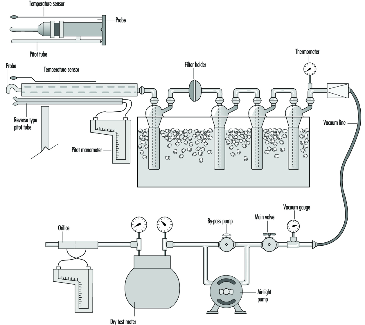
Extractive sampling, particularly isokinetic sampling, can be very accurate and versatile, and has several uses:
- It is a recognized sampling method with adequate quality controls, and thus can be used to determine compliance with standards.
- The potential accuracy of the method makes it suitable for performance testing of new control equipment.
- Since samples can be collected and analysed under controlled laboratory conditions for many components, it is useful for characterizing the gas stream.
A simplified and automated sampling system can be connected to a continuous gas (electrochemical, ultraviolet-photometric or flame ionization sensors) or particulate (nephelometer) analyzer to continuously monitor emissions. This can provide documentation of the emissions, and instantaneous operating status of the air pollution control system.
In situ sampling
Emissions can also be sampled in the stack. Figure 2 is a representation of a simple transmissometer used to measure materials in the gas stream. In this example, a beam of light is projected across the stack to a photocell. The particulates or coloured gas will absorb or block some of the light. The more material, the less light will get to the photocell. (See figure 2.)
Figure 2. A simple transmissometer to measure particulates in a stack
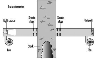
By using different light sources and detectors such as ultraviolet light (UV), gases transparent to visible light can be detected. These devices can be tuned to specific gases, and thus can measure gas concentration in the waste stream.
An in situ monitoring system has an advantage over an extractive system in that it can measure the concentration across the entire stack or duct, whereas the extractive method measures concentrations only at the point from which the sample was extracted. This can result in significant error if the sample gas stream is not well mixed. However, the extractive method offers more methods of analysis, and thus perhaps can be used in more applications.
Since the in situ system provides a continuous readout, it can be used to document emissions, or to fine tune the operating system.
Water Pollution Control
This article is intended to provide the reader with an understanding of currently available technology for approaching water pollution control, building on the discussion of trends and occurrence provided by Hespanhol and Helmer in the chapter Environmental Health Hazards. The following sections address the control of water pollution problems, first under the heading “Surface Water Pollution Control” and then under the heading “Groundwater Pollution Control”.
Surface Water Pollution Control
Definition of water pollution
Water pollution refers to the qualitative state of impurity or uncleanliness in hydrologic waters of a certain region, such as a watershed. It results from an occurrence or process which causes a reduction in the utility of the earth’s waters, especially as related to human health and environmental effects. The pollution process stresses the loss of purity through contamination, which further implies intrusion by or contact with an outside source as the cause. The term tainted is applied to extremely low levels of water pollution, as in their initial corruption and decay. Defilement is the result of pollution and suggests violation or desecration.
Hydrologic waters
The earth’s natural waters may be viewed as a continuously circulating system as shown in figure 1, which provides a graphic illustration of waters in the hydrologic cycle, including both surface and subsurface waters.
Figure 1. The hydrologic cycle

As a reference for water quality, distilled waters (H2O) represent the highest state of purity. Waters in the hydrologic cycle may be viewed as natural, but are not pure. They become polluted from both natural and human activities. Natural degradation effects may result from a myriad of sources - from fauna, flora, volcano eruptions, lightning strikes causing fires and so on, which on a long-term basis are considered to be prevailing background levels for scientific purposes.
Human-made pollution disrupts the natural balance by superimposing waste materials discharged from various sources. Pollutants may be introduced into the waters of the hydrologic cycle at any point. For example: atmospheric precipitation (rainfall) may become contaminated by air pollutants; surface waters may become polluted in the runoff process from watersheds; sewage may be discharged into streams and rivers; and groundwaters may become polluted through infiltration and underground contamination.
Figure 2 shows a distribution of hydrologic waters. Pollution is then superimposed on these waters and may therefore be viewed as an unnatural or unbalanced environmental condition. The process of pollution may occur in waters of any part of the hydrologic cycle, and is more obvious on the earth’s surface in the form of runoff from watersheds into streams and rivers. However groundwater pollution is also of major environmental impact and is discussed following the section on surface water pollution.
Figure 2. Distribution of precipitation
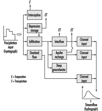
Watershed sources of water pollution
Watersheds are the originating domain of surface water pollution. A watershed is defined as an area of the earth’s surface on which hydrologic waters fall, accumulate, are used, disposed of, and eventually are discharged into streams, rivers or other bodies of water. It is comprised of a drainage system with ultimate runoff or collection in a stream or river. Large river watersheds are usually referred to as drainage basins. Figure 3 is a representation of the hydrologic cycle on a regional watershed. For a region, the disposition of the various waters can be written as a simple equation, which is the basic equation of hydrology as written by Viessman, Lewis and Knapp (1989); typical units are mm/year:
P - R - G - E - T = ±S
where:
P = precipitation (i.e., rainfall, snowfall, hail)
R = runoff or watershed surface flow
G = groundwater
E = evaporation
T = transpiration
S = surface storage
Figure 3. Regional hydrologic cycle
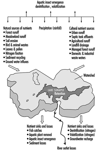
Precipitation is viewed as the initiating form in the above hydrologic budget. The term runoff is synonymous with stream flow. Storage refers to reservoirs or detention systems which collect waters; for example, a human-made dam (barrage) on a river creates a reservoir for purposes of water storage. Groundwater collects as a storage system and may flow from one location to another; it may be influent or effluent in relation to surface streams. Evaporation is a water surface phenomenon, and transpiration is associated with transmission from biota.
Although watersheds may vary greatly in size, certain drainage systems for water pollution designation are classified as urban or non-urban (agricultural, rural, undeveloped) in character. Pollution occurring within these drainage systems originates from the following sources:
Point sources: waste discharges into a receiving water body at a specific location, at a point such as a sewer pipe or some type of concentrated system outlet.
Non-point (dispersed) sources: pollution entering a receiving water body from dispersed sources in the watershed; uncollected rainfall runoff water drainage into a stream is typical. Non-point sources are also sometimes referred to as “diffuse” waters; however, the term dispersed is seen as more descriptive.
Intermittent sources: from a point or source which discharges under certain circumstances, such as with overloaded conditions; combined sewer overflows during heavy rainfall runoff periods are typical.
Water pollutants in streams and rivers
When deleterious waste materials from the above sources are discharged into streams or other bodies of water, they become pollutants which have been classified and described in a previous section. Pollutants or contaminants which enter a body of water can be further divided into:
- degradable (non-conservative) pollutants: impurities which eventually decompose into harmless substances or which may be removed by treatment methods; that is, certain organic materials and chemicals, domestic sewage, heat, plant nutrients, most bacteria and viruses, certain sediments
- non-degradable (conservative) pollutants: impurities which persist in the water environment and do not reduce in concentration unless diluted or removed through treatment; that is, certain organic and inorganic chemicals, salts, colloidal suspensions
- hazardous waterborne pollutants: complex forms of deleterious wastes including toxic trace metals, certain inorganic and organic compounds
- radionuclide pollutants: materials which have been subjected to a radioactive source.
Water pollution control regulations
Broadly applicable water pollution control regulations are generally promulgated by national governmental agencies, with more detailed regulations by states, provinces, municipalities, water districts, conservation districts, sanitation commissions and others. At the national and state (or province) levels, environmental protection agencies (EPAs) and ministries of health are usually charged with this responsibility. In the discussion of regulations below, the format and certain portions follow the example of the water quality standards currently applicable for the US State of Ohio.
Water quality use designations
The ultimate goal in the control of water pollution would be zero discharge of pollutants to water bodies; however, complete achievement of this objective is usually not cost effective. The preferred approach is to set limitations on waste disposal discharges for the reasonable protection of human health and the environment. Although these standards may vary widely in different jurisdictions, use designations for specific bodies of water are commonly the basis, as briefly addressed below.
Water supplies include:
- public water supply: waters which with conventional treatment will be suitable for human consumption
- agricultural supply: waters suitable for irrigation and livestock watering without treatment
- industrial/commercial supply: waters suitable for industrial and commercial uses with or without treatment.
Recreational activities include:
- bathing waters: waters which during certain seasons are suitable for swimming as approved for water quality along with protective conditions and facilities
- primary contact: waters which during certain seasons are suitable for full body contact recreation such as swimming, canoeing and underwater diving with minimal threat to public health as a result of water quality
- secondary contact: waters which during certain seasons are suitable for partial body contact recreation such as, but not limited to, wading, with minimal threat to public health as a result of water quality.
Public water resources are categorized as water bodies which lie within park systems, wetland, wildlife areas, wild, scenic and recreational rivers and publicly owned lakes, and waters of exceptional recreational or ecological significance.
Aquatic life habitats
Typical designations will vary according to climates, but relate to conditions in water bodies for supporting and maintaining certain aquatic organisms, especially various species of fish. For example, use designations in a temperate climate as subdivided in regulations for the State of Ohio Environmental Protection Agency (EPA) are listed below without detailed descriptions:
- warmwater
- limited warmwater
- exceptional warmwater
- modified warmwater
- seasonal salmonid
- coldwater
- limited resource water.
Water pollution control criteria
Natural waters and wastewaters are characterized in terms of their physical, chemical and biological composition. The principal physical properties and the chemical and biological constituents of wastewater and their sources are a lengthy list, reported in a textbook by Metcalf and Eddy (1991). Analytical methods for these determinations are given in a widely used manual entitled Standard Methods for the Examination of Water and Waste Water by the American Public Health Association (1995).
Each designated water body should be controlled according to regulations which may be comprised of both basic and more detailed numerical criteria as briefly discussed below.
Basic freedom from pollution. To the extent practical and possible, all bodies of water should attain the basic criteria of the “Five Freedoms from Pollution”:
- free from suspended solids or other substances that enter the waters as a result of human activity and that will settle to form putrid or otherwise objectionable sludge deposits, or that will adversely affect aquatic life
- free from floating debris, oil, scum and other floating materials entering the waters as a result of human activity in amounts sufficient to be unsightly or cause degradation
- free from materials entering the waters as a result of human activity, producing colour, odour or other conditions in such degree as to create a nuisance
- free from substances entering the waters as a result of human activity, in concentrations that are toxic or harmful to human, animal or aquatic life and/or are rapidly lethal in the mixing zone
- free from nutrients entering the waters as a result of human activity, in concentrations that create nuisance growths of aquatic weeds and algae.
Water quality criteria are numerical limitations and guidelines for the control of chemical, biological and toxic constituents in bodies of water.
With over 70,000-plus chemical compounds in use today it is impractical to specify the control of each. However, criteria for chemicals can be established on the basis of limitations as they first of all relate to three major classes of consumption and exposure:
Class 1: Chemical criteria for protection of human health are of first major concern and should be set according to recommendations from governmental health agencies, the WHO and recognized health research organizations.
Class 2: Chemical criteria for control of agricultural water supply should be based on recognized scientific studies and recommendations which will protect against adverse effects on crops and livestock as a result of crop irrigation and livestock watering.
Class 3: Chemical criteria for protection of aquatic life should be based on recognized scientific studies regarding the sensitivity of these species to specific chemicals and also as related to human consumption of fish and sea foods.
Wastewater effluent criteria relate to limitations on pollutant constituents present in wastewater effluents and are a further method of control. They may be set as related to the water use designations of bodies of water and as they relate to the above classes for chemical criteria.
Biological criteria are based on water body habitat conditions which are needed to support aquatic life.
Organic content of wastewaters and natural waters
The gross content of organic matter is most important in characterizing the pollutional strength of both wastewater and natural waters. Three laboratory tests are commonly used for this purpose:
Biochemical oxygen demand (BOD): five-day BOD (BOD5) is the most widely used parameter; this test measures the dissolved oxygen used by micro-organisms in the biochemical oxidation of organic matter over this period.
Chemical oxygen demand (COD): this test is to measure the organic matter in municipal and industrial wastes that contain compounds that are toxic to biological life; it is a measure of the oxygen equivalent of the organic matter that can be oxidized.
Total organic carbon (TOC): this test is especially applicable to small concentrations of organic matter in water; it is a measure of the organic matter that is oxidized to carbon dioxide.
Antidegradation policy regulations
Antidegradation policy regulations are a further approach for preventing the spread of water pollution beyond certain prevailing conditions. As an example, the Ohio Environmental Protection Agency Water Quality Standards antidegradation policy consists of three tiers of protection:
Tier 1: Existing uses must be maintained and protected. No further water quality degradation is allowed that would interfere with existing designated uses.
Tier 2: Next, water quality better than that needed to protect uses must be maintained unless it is shown that a lower water quality is necessary for important economic or social development, as determined by the EPA Director.
Tier 3: Finally, the quality of water resource waters must be maintained and protected. Their existing ambient water quality is not to be degraded by any substances determined to be toxic or to interfere with any designated use. Increased pollutant loads are allowed to be discharged into water bodies if they do not result in lowering existing water quality.
Water pollution discharge mixing zones and waste load allocation modelling
Mixing zones are areas in a body of water which allow for treated or untreated wastewater discharges to attain stabilized conditions, as illustrated in figure 4 for a flowing stream. The discharge is initially in a transitory state which becomes progressively diluted from the source concentration to the receiving water conditions. It is not to be considered as a treatment entity and may be delineated with specific restrictions.
Figure 4. Mixing zones
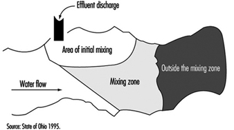
Typically, mixing zones must not:
- interfere with migration, survival, reproduction or growth of aquatic species
- include spawning or nursery areas
- include public water supply intakes
- include bathing areas
- constitute more than 1/2 the width of a stream
- constitute more than 1/2 the cross-sectional area of a stream mouth
- extend downstream for a distance more than five times the stream width.
Waste load allocation studies have become important because of the high cost of nutrient control of wastewater discharges to avoid instream eutrophication (defined below). These studies generally employ the use of computer models for simulation of water quality conditions in a stream, particularly with regard to nutrients such as forms of nitrogen and phosphorous, which affect the dissolved oxygen dynamics. Traditional water quality models of this type are represented by the US EPA model QUAL2E, which has been described by Brown and Barnwell (1987). A more recent model proposed by Taylor (1995) is the Omni Diurnal Model (ODM), which includes a simulation of the impact of rooted vegetation on instream nutrient and dissolved oxygen dynamics.
Variance provisions
All water pollution control regulations are limited in perfection and therefore should include provisions which allow for judgemental variance based on certain conditions which may prevent immediate or complete compliance.
Risk assessment and management as related to water pollution
The above water pollution control regulations are typical of worldwide governmental approaches for achieving compliance with water quality standards and wastewater effluent discharge limits. Generally these regulations have been set on the basis of health factors and scientific research; where some uncertainty exists as to possible effects, safety factors often are applied. Implementation of certain of these regulations may be unreasonable and exceedingly costly for the public at large as well as for private enterprise. Therefore there is a growing concern for more efficient allocation of resources in achieving goals for water quality improvement. As previously pointed out in the discussion of hydrologic waters, pristine purity does not exist even in naturally occurring waters.
A growing technological approach encourages assessment and management of ecological risks in the setting of water pollution regulations. The concept is based on an analysis of the ecological benefits and costs in meeting standards or limits. Parkhurst (1995) has proposed the application of aquatic ecological risk assessment as an aid in setting water pollution control limits, particularly as applicable for the protection of aquatic life. Such risk assessment methods may be applied to estimate the ecological effects of chemical concentrations for a broad range of surface water pollution conditions including:
- point source pollution
- non-point source pollution
- existing contaminated sediments in stream channels
- hazardous wastes sites as related to water bodies
- analysis of existing water pollution control criteria.
The proposed method consists of three tiers; as shown in figure 5 which illustrates the approach.
Figure 5. Methods for conducting risk assessment for successive tiers of analysis. Tier 1: Screening level; Tier 2: Quantification of potentially significant risks ; Tier 3: Site-specific risk quantification
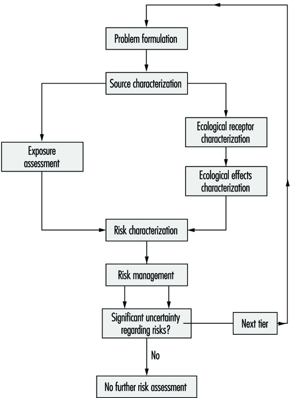
Water pollution in lakes and reservoirs
Lakes and reservoirs provide for the volumetric storage of watershed inflow and may have long flushing time periods as compared with the rapid inflow and outflow for a reach in a flowing stream. Therefore they are of special concern with regard to the retention of certain constituents, especially nutrients including forms of nitrogen and phosphorous which promote eutrophication. Eutrophication is a natural ageing process in which the water content becomes organically enriched, leading to the domination of undesirable aquatic growth, such as algae, water hyacinth and so on. The eutrophic process tends to decrease aquatic life and has detrimental dissolved oxygen effects. Both natural and cultural sources of nutrients may promote the process, as illustrated by Preul (1974) in figure 6, showing a schematic listing of nutrient sources and sinks for Lake Sunapee, in the US State of New Hampshire.
Figure 6. Schematic listing of nutrient (nitrogen and phosphorus) sources and sinks for Lake Sunapee, New Hampshire (US)
Lakes and reservoirs, of course, can be sampled and analysed to determine their trophic status. Analytical studies usually start with a basic nutrient balance such as the following:
(lake influent nutrients) = (lake effluent nutrients) + (nutrient retention in lake)
This basic balance can be further expanded to include the various sources shown in figure 6.
Flushing time is an indication of the relative retention aspects of a lake system. Shallow lakes, such as Lake Erie, have relatively short flushing times and are associated with advanced eutrophication because shallow lakes often are more conducive to aquatic plant growth. Deep lakes such as Lake Tahoe and Lake Superior have very long flushing periods, which are usually associated with lakes with minimal eutrophication because up to the present time, they have not been overloaded and also because their extreme depths are not conducive to extensive aquatic plant growth except in the epilimnion (upper zone). Lakes in this category are generally classified as oligotrophic, on the basis that they are relatively low in nutrients and support minimal aquatic growth such as algae.
It is of interest to compare the flushing times of some major US lakes as reported by Pecor (1973) using the following calculation basis:
lake flushing time (LFT) = (lake storage volume)/(lake outflow)
Some examples are: Lake Wabesa (Michigan), LFT=0.30 years; Houghton Lake (Michigan), 1.4 years; Lake Erie, 2.6 years; Lake Superior, 191 years; Lake Tahoe, 700 years.
Although the relationship between the process of eutrophication and nutrient content is complex, phosphorous is typically recognized as the limiting nutrient. Based on fully mixed conditions, Sawyer (1947) reported that algal blooms tend to occur if nitrogen values exceed 0.3 mg/l and phosphorous exceeds 0.01 mg/l. In stratified lakes and reservoirs, low dissolved oxygen levels in the hypoliminion are early signs of eutrophication. Vollenweider (1968, 1969) has developed critical loading levels of total phosphorous and total nitrogen for a number of lakes based on nutrient loadings, mean depths and trophic states. For a comparison of work on this subject, Dillon (1974) has published a critical review of Vollenweider’s nutrient budget model and other related models. More recent computer models are also available for simulating nitrogen/phosphorous cycles with temperature variations.
Water pollution in estuaries
An estuary is an intermediate passageway of water between the mouth of a river and a sea coast. This passageway is comprised of a river mouth channel reach with river inflow (fresh water) from upstream and outflow discharge on the downstream side into a constantly changing tailwater level of sea water (salt water). Estuaries are continuously affected by tidal fluctuations and are among the most complex bodies of water encountered in water pollution control. The dominant features of an estuary are variable salinity, a salt wedge or interface between salt and fresh water, and often large areas of shallow, turbid water overlying mud flats and salt marshes. Nutrients are largely supplied to an estuary from the inflowing river and combine with the sea water habitat to provide prolific production of biota and sea life. Especially desired are seafoods harvested from estuaries.
From a water pollution standpoint, estuaries are individually complex and generally require special investigations employing extensive field studies and computer modelling. For a further basic understanding, the reader is referred to Reish 1979, on marine and estuarine pollution; and to Reid and Wood 1976, on the ecology of inland waters and estuaries.
Water pollution in marine environments
Oceans may be viewed as the ultimate receiving water or sink, since wastes carried by rivers finally discharge into this marine environment. Although oceans are vast bodies of salt water with seemingly unlimited assimilation capacity, pollution tends to blight coastlines and further affects marine life.
Sources of marine pollutants include many of those encountered in land-based wastewater environments plus more as related to marine operations. A limited list is given below:
- domestic sewage and sludge, industrial wastes, solid wastes, shipboard wastes
- fishery wastes, sediments and nutrients from rivers and land runoff
- oil spills, offshore oil exploration and production wastes, dredge operations
- heat, radioactive wastes, waste chemicals, pesticides and herbicides.
Each of the above requires special handling and methods of control. The discharge of domestic sewage and sewage sludges through ocean outfalls is perhaps the major source of marine pollution.
For current technology on this subject, the reader is referred to the book on marine pollution and its control by Bishop (1983).
Techniques for reducing pollution in wastewater discharges
Large-scale wastewater treatment is typically carried out by municipalities, sanitary districts, industries, commercial enterprises and various pollution control commissions. The purpose here is to describe contemporary methods of municipal wastewater treatment and then to provide some insights regarding treatment of industrial wastes and more advanced methods.
In general, all processes of wastewater treatment may be grouped into physical, chemical or biological types, and one or more of these may be employed to achieve a desired effluent product. This classification grouping is most appropriate in the understanding of wastewater treatment approaches and is tabulated in table 1.
Table 1. General classification of wastewater treatment operations and processes
|
Physical Operations |
Chemical Processes |
Biological Processes |
|
Flow measurement |
Precipitation |
Aerobic action |
Contemporary methods of wastewater treatment
The coverage here is limited and is intended to provide a conceptual overview of current wastewater treatment practices around the world rather than detailed design data. For the latter, the reader is referred to Metcalf and Eddy 1991.
Municipal wastewaters along with some intermingling of industrial/commercial wastes are treated in systems commonly employing primary, secondary and tertiary treatment as follows:
Primary treatment system: Pre-treat ® Primary settling ® Disinfection (chlorination) ® Effluent
Secondary treatment system: Pre-treat ® Primary settling ® Biological unit ® Second settling ® Disinfection (chlorination) ® Effluent to stream
Tertiary treatment system: Pre-treat ® Primary settling ® Biological unit ® Second settling ® Tertiary unit ® Disinfection (chlorination) ® Effluent to stream
Figure 7 further shows a schematic diagram of a conventional wastewater treatment system. Overview descriptions of the above processes follow.
Figure 7. Schematic diagram of conventional wastewater treatment
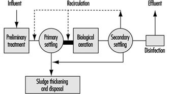
Primary treatment
The basic objective of primary treatment for municipal wastewaters, including domestic sewage intermingled with some industrial/commercial wastes, is to remove suspended solids and clarify the wastewater, to make it suitable for biological treatment. After some pre-treatment handling such as screening, grit removal and comminution, the main process of primary sedimentation is the settling of the raw wastewater in large settling tanks for periods up to several hours. This process removes from 50 to 75% of the total suspended solids, which are drawn off as an underflow sludge collected for separate treatment. The overflow effluent from the process then is directed for secondary treatment. In certain cases, chemicals may be employed to improve the degree of primary treatment.
Secondary treatment
The portion of the organic content of the wastewater which is finely suspended or dissolved and not removed in the primary process, is treated by secondary treatment. The generally accepted forms of secondary treatment in common use include trickling filters, biological contactors such as rotating discs, activated sludge, waste stabilization ponds, aerated pond systems and land application methods, including wetland systems. All of these systems will be recognized as employing biological processes of some form or another. The most common of these processes are briefly discussed below.
Biological contactor systems. Trickling filters are one of the earliest forms of this method for secondary treatment and are still widely used with some improved methods of application. In this treatment, the effluent from the primary tanks is applied uniformly onto a bed of media, such as rock or synthetic plastic media. Uniform distribution is accomplished typically by trickling the liquid from perforated piping rotated over the bed intermittently or continuously according to the desired process. Depending on the rate of organic and hydraulic loadings, trickling filters can remove up to 95% of the organic content, usually analysed as biochemical oxygen demand (BOD). There are numerous other more recent biological contactor systems in use which can provide treatment removals in the same range; some of these methods offer special advantages, particularly applicable in certain limiting conditions such as space, climate and so on. It is to be noted that a following secondary settling tank is considered to be a necessary part of completing the process. In secondary settling, some so-called humus sludge is drawn off as an underflow, and the overflow is discharged as a secondary effluent.
Activated sludge. In the most common form of this biological process, primary treated effluent flows into an activated sludge unit tank containing a previously existing biological suspension called activated sludge. This mixture is referred to as mixed liquor suspended solids (MLSS) and is provided a contact period typically ranging from several hours up to 24 hours or more, depending on the desired results. During this period the mixture is highly aerated and agitated to promote aerobic biological activity. As the process finalizes, a portion of the mixture (MLSS) is drawn off and returned to the influent for continuation of the biological activation process. Secondary settling is provided following the activated sludge unit for the purpose of settling out the activated sludge suspension and discharging a clarified overflow as an effluent. The process is capable of removing up to about 95% of the influent BOD.
Tertiary treatment
A third level of treatment may be provided where a higher degree of pollutant removal is required. This form of treatment may typically include sand filtration, stabilization ponds, land disposal methods, wetlands and other systems which further stabilize the secondary effluent.
Disinfection of effluents
Disinfection is commonly required to reduce bacteria and pathogens to acceptable levels. Chlorination, chlorine dioxide, ozone and ultraviolet light are the most commonly used processes.
Overall wastewater treatment plant efficiency
Wastewaters include a broad range of constituents which generally are classified as suspended and dissolved solids, inorganic constituents and organic constituents.
The efficiency of a treatment system can be measured in terms of the percentage removal of these constituents. Common parameters of measurement are:
- BOD: biochemical oxygen demand, measured in mg/l
- COD: chemical oxygen demand, measured in mg/l
- TSS: total suspended solids, measured in mg/l
- TDS: total dissolved solids, measured in mg/l
- nitrogen forms: including nitrate and ammonia, measured in mg/l (nitrate is of particular concern as a nutrient in eutrophication)
- phosphate: measured in mg/l (also of particular concern as a nutrient in eutrophication)
- pH: degree of acidity, measured as a number from 1 (most acid) to 14 (most alkaline)
- coliform bacteria counts: measured as most probable number per 100 ml (Escherichia and fecal coliform bacteria are most common indicators).
Industrial wastewater treatment
Types of industrial wastes
Industrial (non-domestic) wastes are numerous and vary greatly in composition; they may be highly acidic or alkaline, and often require a detailed laboratory analysis. Specialized treatment may be necessary to render them innocuous before discharge. Toxicity is of great concern in the disposal of industrial wastewaters.
Representative industrial wastes include: pulp and paper, slaughterhouse, brewery, tannery, food processing, cannery, chemical, petroleum, textile, sugar, laundry, meat and poultry, hog feeding, rendering and many others. The initial step in treatment design development is an industrial waste survey, which provides data on variations in flow and waste characteristics. Undesirable waste characteristics as listed by Eckenfelder (1989) can be summarized as follows:
- soluble organics causing depletion of dissolved oxygen
- suspended solids
- trace organics
- heavy metals, cyanide and toxic organics
- colour and turbidity
- nitrogen and phosphorus
- refractory substances resistant to biodegradation
- oil and floating material
- volatile materials.
The US EPA has further defined a list of toxic organic and inorganic chemicals with specific limitations in granting discharge permits. The list includes more than 100 compounds and is too long to reprint here, but may be requested from the EPA.
Treatment methods
The handling of industrial wastes is more specialized than the treatment of domestic wastes; however, where amenable to biological reduction, they are usually treated using methods similar to those previously described (secondary/tertiary biological treatment approaches) for municipal systems.
Waste stabilization ponds are a common method of organic wastewater treatment where sufficient land area is available. Flow-through ponds are generally classified according to their bacterial activity as aerobic, facultative or anaerobic. Aerated ponds are supplied with oxygen by diffused or mechanical aeration systems.
Figure 8 and figure 9 show sketches of waste stabilization ponds.
Figure 8. Two-cell stabilization pond: cross sectional diagram

Figure 9. Aerated lagoon types: schematic diagram

Pollution prevention and waste minimization
When industrial waste in-plant operations and processes are analysed at their source, they often can be controlled so as to prevent significant polluting discharges.
Recirculation techniques are important approaches in pollution prevention programmes. A case study example is a recycling plan for a leather tannery wastewater effluent published by Preul (1981), which included chrome recovery/reuse along with the complete recirculation of all tannery wastewaters with no effluent to any stream except in emergencies. The flow diagram for this system is shown in figure 10.
Figure 10. Flow diagram for tannery wastewater effluent recycling system
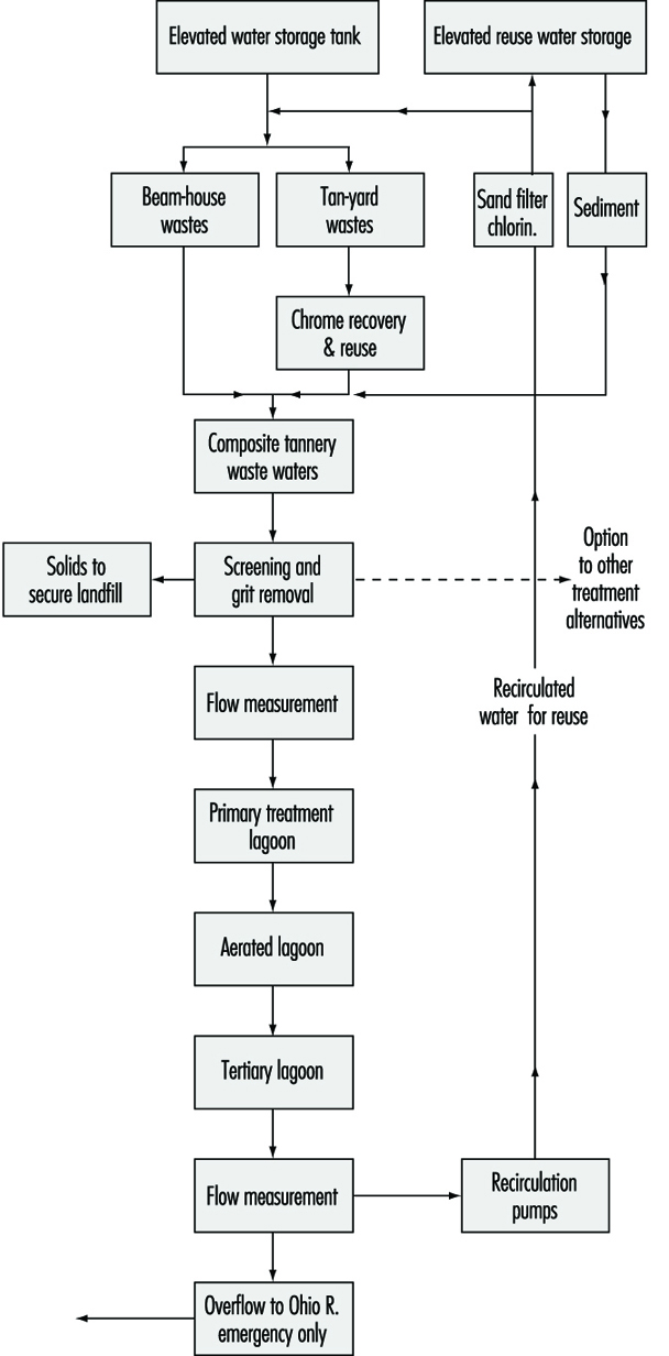
For more recent innovations in this technology, the reader is referred to a publication on pollution prevention and waste minimization by the Water Environment Federation (1995).
Advanced methods of wastewater treatment
A number of advanced methods are available for higher degrees of removal of pollution constituents as may be required. A general listing includes:
filtration (sand and multimedia)
chemical precipitation
carbon adsorption
electrodialysis
distillation
nitrification
algae harvesting
reclamation of effluents
micro-straining
ammonia stripping
reverse osmosis
ion exchange
land application
denitrification
wetlands.
The most appropriate process for any situation must be determined on the basis of the quality and quantity of the raw wastewater, the receiving water requirements and, of course, costs. For further reference, see Metcalf and Eddy 1991, which includes a chapter on advanced wastewater treatment.
Advanced wastewater treatment case study
The case study of the Dan Region Sewage Reclamation Project discussed elsewhere in this chapter provides an excellent example of innovative methods for wastewater treatment and reclamation.
Thermal pollution
Thermal pollution is a form of industrial waste, defined as deleterious increases or reductions in normal water temperatures of receiving waters caused by the disposal of heat from human-made facilities. The industries producing major waste heat are fossil fuel (oil, gas and coal) and nuclear power generating plants, steel mills, petroleum refineries, chemical plants, pulp and paper mills, distilleries and laundries. Of particular concern is the electric power generating industry which supplies energy for many countries (e.g., about 80% in the US).
Impact of waste heat on receiving waters
Influence on waste assimilation capacity
- Heat increases biological oxidation.
- Heat decreases oxygen saturation content of water and decreases rate of natural reoxygenation.
- The net effect of heat is generally detrimental during warm months of year.
- Winter effect may be beneficial in colder climates, where ice conditions are broken up and surface aeration is provided for fish and aquatic life.
Influence on aquatic life
Many species have temperature tolerance limits and need protection, particularly in heat affected reaches of a stream or body of water. For example, cold water streams usually have the highest type of sport fish such as trout and salmon, whereas warm waters generally support coarse fish populations, with certain species such as pike and bass fish in intermediate temperature waters.
Figure 11. Heat exchange at the boundaries of a receiving water cross section
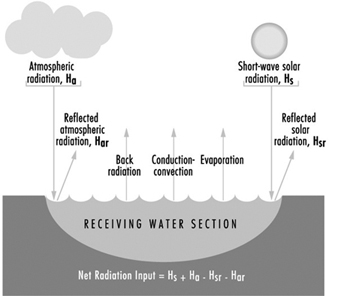
Thermal analysis in receiving waters
Figure 11 illustrates the various forms of natural heat exchange at the boundaries of a receiving water. When heat is discharged to a receiving water such as a river, it is important to analyse the river capacity for thermal additions. The temperature profile of a river can be calculated by solving a heat balance similar to that used in calculating dissolved oxygen sag curves. The principal factors of the heat balance are illustrated in figure 12 for a river reach between points A and B. Each factor requires an individual calculation dependent on certain heat variables. As with a dissolved oxygen balance, the temperature balance is simply a summation of temperature assets and liabilities for a given section. Other more sophisticated analytical approaches are available in the literature on this subject. The results from the heat balance calculations can be used in establishing heat discharge limitations and possibly certain use constraints for a body of water.
Figure 12. River capacity for thermal additions
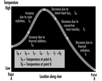
Thermal pollution control
The main approaches for the control of thermal pollution are:
- improved power plant operation efficiencies
- cooling towers
- isolated cooling ponds
- consideration of alternative methods of power generation such as hydro-power.
Where physical conditions are favourable within certain environmental limits, hydro-electric power should be considered as an alternative to fossil-fuel or nuclear power generation. In hydro-electric power generation, there is no disposal of heat and there is no discharge of waste waters causing water pollution.
Groundwater Pollution Control
Importance of groundwater
Since the world’s water supplies are widely extracted from aquifers, it is most important that these sources of supply be protected. It is estimated that more than 95% of the earth’s available fresh water supply is underground; in the United States approximately 50% of the drinking water comes from wells, according to the 1984 US Geological Survey. Because underground water pollution and movement are of subtle and unseen nature, less attention sometimes is given to the analysis and control of this form of water degradation than to surface water pollution, which is far more obvious.
Figure 13. Hydrologic cycle and sources of groundwater contamination

Sources of underground pollution
Figure 13 shows the hydrologic cycle with superimposed sources of groundwater contamination. A complete listing of the potential sources of underground pollution is extensive; however, for illustration the most obvious sources include:
- industrial waste discharges
- polluted streams in contact with aquifers
- mining operations
- solid and hazardous waste disposal
- underground storage tanks such as for petroleum
- irrigation systems
- artificial recharge
- sea water encroachment
- spills
- polluted ponds with permeable bottoms
- disposal wells
- septic tank tile fields and leaching pits
- improper well drilling
- agricultural operations
- roadway de-icing salts.
Specific pollutants in underground contamination are further categorized as:
- undesirable chemical constituents (typical, not complete list) - organic and inorganic (e.g., chloride, sulphate, iron, manganese, sodium, potassium)
- total hardness and total dissolved solids
- toxic constituents (typical, not complete list) - nitrate, arsenic, chromium, lead, cyanide, copper, phenols, dissolved mercury
- undesirable physical characteristics - taste, colour and odour
- pesticides and herbicides - chlorinated hydrocarbons and others
- radioactive materials - various forms of radioactivity
- biological - bacteria, viruses, parasites and so on
- acid (low pH) or caustic (high pH).
Of the above, nitrates are of special concern in both ground waters and surface waters. In groundwater supplies, nitrates can cause the disease methaemoglobinaemia (infant cyanosis). They further cause detrimental eutrophication effects in surface waters and occur in a wide range of water resources, as reported by Preul (1991). Preul (1964, 1967, 1972) and Preul and Schroepfer (1968) have also reported on the underground movement of nitrogen and other pollutants.
Pollution travel in underground domain
Groundwater movement is exceedingly slow and subtle as compared with the travel of surface waters in the hydrologic cycle. For a simple understanding of the travel of ordinary groundwater under ideal steady flow conditions, Darcy’s Law is the basic approach for the evaluation of groundwater movement at low Reynolds numbers (R):
V = K(dh/dl)
where:
V = velocity of groundwater in aquifer, m/day
K = coefficient of permeability of aquifer
(dh/dl) = hydraulic gradient which represents the driving force for movement.
In pollutant travel underground, ordinary groundwater (H2O) is generally the carrying fluid and can be calculated to move at a rate according to the parameters in Darcy’s Law. However, the rate of travel or velocity of a pollutant, such as an organic or inorganic chemical, may be different due to advection and hydrodynamic dispersion processes. Certain ions move slower or faster than the general rate of groundwater flow as a result of reactions within the aquifer media, so that they can be categorized as “reacting” or “non-reacting”. Reactions are generally of the following forms:
- physical reactions between the pollutant and the aquifer and/or the transporting liquid
- chemical reactions between the pollutant and the aquifer and/or the transporting liquid
- biological actions on the pollutant.
The following are typical of reacting and non-reacting underground pollutants:
- reacting pollutants - chromium, ammonium ion, calcium, sodium, iron and so on; cations in general; biological constituents; radioactive constituents
- non-reacting pollutants - chloride, nitrate, sulphate and so on; certain anions; certain pesticide and herbicide chemicals.
At first, it might seem that reacting pollutants are the worst type, but this may not always be the case because the reactions detain or retard pollutant travel concentrations whereas non-reacting pollutant travel may be largely uninhibited. Certain “soft” domestic and agricultural products are now available which biologically degrade after a period of time and therefore avoid the possibility of groundwater contamination.
Aquifer remediation
Prevention of underground pollution is obviously the best approach; however, uncontrolled existence of polluted groundwater conditions usually is made known after its occurrence, such as by complaints from water well users in the area. Unfortunately, by the time the problem is recognized, severe damage may have occurred and remediation is necessary. Remediation may require extensive hydro-geological field investigations with laboratory analyses of water samples in order to establish the extent of pollutant concentrations and travel plumes. Often existing wells can be used in initial sampling, but severe cases may require extensive borings and water samplings. These data can then be analysed to establish current conditions and to make future condition predictions. The analysis of groundwater contamination travel is a specialized field often requiring the use of computer models to better understand the groundwater dynamics and to make predictions under various constraints. A number of two- and three-dimensional computer models are available in the literature for this purpose. For more detailed analytical approaches, the reader is referred to the book by Freeze and Cherry (1987).
Pollution prevention
The preferred approach for the protection of groundwater resources is pollution prevention. Although drinking water standards generally apply to the use of groundwater supplies, the raw water supplies require protection from contamination. Governmental entities such as ministries of health, natural resources agencies, and environmental protection agencies are generally responsible for such activities. Groundwater pollution control efforts are largely directed at protection of aquifers and the prevention of pollution.
Pollution prevention requires land-use controls in the form of zoning and certain regulations. Laws may apply to the prevention of specific functions as particularly applicable to point sources or actions which potentially may cause pollution. Control by land-use zoning is a groundwater protection tool which is most effective at the municipal or county level of government. Aquifer and wellhead protection programmes as discussed below are leading examples of pollution prevention.
An aquifer protection programme requires establishing the boundaries of the aquifer and its recharge areas. Aquifers may be of an unconfined or confined type, and therefore need to be analysed by a hydrologist to make this determination. Most major aquifers are generally well known in developed countries, but other areas may require field investigations and hydrogeologic analysis. The key element of the programme in the protection of the aquifer from water quality degradation is control of land use over the aquifer and its recharge areas.
Wellhead protection is a more definitive and limited approach which applies to the recharge area contributing to a particular well. The US federal government by amendments passed in 1986 to the Safe Drinking Water Act (SDWA) (1984) now requires that specific wellhead protection areas be established for public supply wells. The wellhead protection area (WHPA) is defined in the SDWA as “the surface and subsurface area surrounding a water well or well field, supplying a public water supply system, through which contaminants are reasonably likely to move toward and reach such water well or well field.” The main objective in the WHPA programme, as outlined by the US EPA (1987), is the delineation of well protection areas based on selected criteria, well operation and hydrogeologic considerations.
Dan Region Sewage Reclamation Project: A Case Study
Conception and Design
The Dan Region Reclamation Project of municipal wastewater is the biggest project of its kind in the world. It consists of facilities for treatment and groundwater recharge of municipal wastewater from the Dan Region Metropolitan Area - an eight-city conglomerate centred around Tel Aviv, Israel, with a combined population of about 1.5 million inhabitants. The project was created for the purpose of collection, treatment and disposal of municipal wastewater. The reclaimed effluent, after a relatively long detention period in the underground aquifer, is pumped for unrestricted agricultural use, irrigating the arid Negev (the southern part of Israel). A general scheme of the project is given in figure 1. The project was established in the 1960s, and has been growing continuously. At present, the system collects and treats about 110 x 106 m3 per year. Within a few years, at its final stage, the system will handle 150 to 170 x 106 m3 per year.
Figure 1. Dan Region Sewage Reclamation Plant: layout
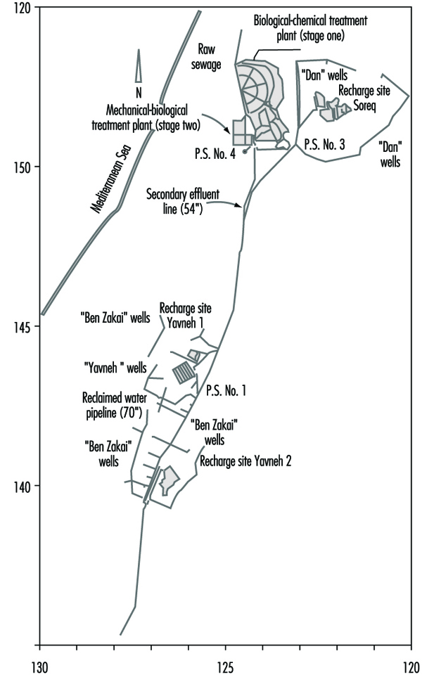
Sewage treatment plants are known to create a multitude of environmental and occupational health problems. The Dan Region project is a unique system of national importance that combines national benefit together with considerable saving of water resources, high treatment efficiency and production of inexpensive water, without creating excessive occupational hazards.
Throughout the design, installation and routine operation of the system, careful consideration has been given to water sanitation and occupational hygiene concerns. All necessary precautions have been taken to ensure that the reclaimed wastewater will be practically as safe as regular drinking water, in the event that people accidentally drink or swallow it. Similarly, appropriate attention has been given to the issue of reducing to the minimum any potential exposure to accidents or other biological, chemical or physical hazards that may affect either the workers at the wastewater treatment plant proper or other workers engaged in the disposal and agricultural use of the reclaimed water.
At Stage One of the project, the wastewater was biologically treated by a system of facultative oxidation ponds with recirculation and additional chemical treatment by a lime-magnesium process, followed by detention of the high-pH effluent in “polishing ponds”. The partially treated effluent was recharged to the regional groundwater aquifer by means of the Soreq spreading basins.
At Stage Two, the wastewater conveyed to the treatment plant undergoes mechanical-biological treatment by means of an activated-sludge process with nitrification-denitrification. The secondary effluent is recharged to the groundwater by means of the spreading basins Yavneh 1 and Yavneh 2.
The complete system consists of a number of different elements complementing each other:
- a wastewater treatment plant system, comprised of an activated-sludge plant (the biomechanical plant), which treats most of the wastes, and of a system of oxidation and polishing ponds used mostly for treatment of excess sewage flows
- a groundwater recharge system for the treated effluent, which consists of spreading basins, at two different sites (Yavneh and Soreq), that are intermittently flooded; the absorbed effluent passes through the soil’s unsaturated zone and through a portion of the aquifer, and creates a special zone that is dedicated to complementary effluent treatment and seasonal storage, which is called SAT (soil-aquifer-treatment)
- networks of observation wells (53 wells all together) which surround the recharge basins and allow the monitoring of the efficiency of the treatment process
- networks of recovery wells (a total of 74 active wells in 1993) which surround the recharge sites
- a special and separate reclaimed water conveyance main for unrestricted irrigation of agricultural areas in the Negev; this main is called “The Third Negev Line”, and it complements the water supply system to the Negev, which includes another two major fresh water supply main lines
- a setup for chlorination of the effluent, which consists, at present, of three chlorination sites (two more to be added in the future)
- six operational reservoirs along the conveyance system, which regulate the amounts of water pumped and consumed along the system
- an effluent distribution system, composed of 13 major pressure zones, along the effluent main, that supply the treated water to the consumers
- a comprehensive monitoring system which supervises and controls the complete operation of the project.
Description of the Reclamation System
The general scheme of the reclamation system is presented in figure 1 and the flow diagram in figure 2. The system consists of the following segments: wastewater treatment plant, water recharge fields, recovery wells, conveyance and distribution system, chlorination setup and a comprehensive monitoring system.
Figure 2. Flow diagram of Dan Region Project
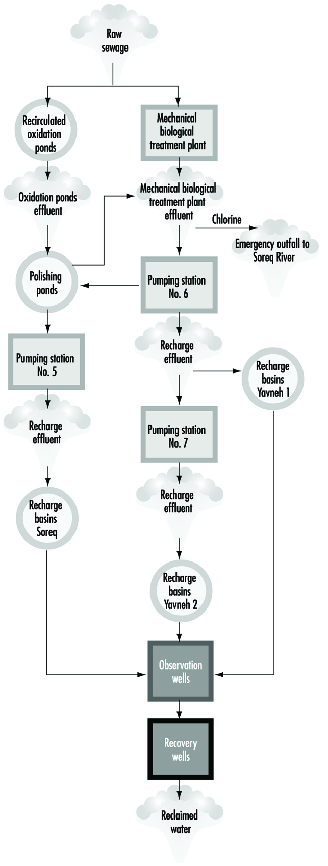
The wastewater treatment plant
The wastewater treatment plant of the Dan Region Metropolitan Area receives the domestic wastes of the eight cities in the region, and also handles part of their industrial wastes. The plant is located within the Rishon-Lezion sand dunes and is based mostly on secondary treatment of the wastes by the activated-sludge method. Some of the wastes, mostly during peak-flow discharges, are treated in another, older system of oxidation ponds occupying an area of 300 acres. The two systems together can handle, at present, about 110 x 106 m3 per year.
The recharge fields
The treatment plant effluents are pumped into three different sites located within the regional sand dunes, where they are spread on the sand and percolate downward into the underground aquifer for temporary storage and for additional time-dependent treatment. Two of the spreading basins are used for recharge of the mechanical-biological treatment-plant effluent. These are Yavneh 1 (60 acres, located 7 km to the south of the plant) and Yavneh 2 (45 acres, 10 km south of the plant); the third basin is used for recharge of a mixture of the oxidation ponds effluent and a certain fraction from the biomechanical treatment plant that is required in order to improve the quality of the effluent to the necessary level. This is the Soreq site, which has an area of about 60 acres and is located to the east of the ponds.
The recovery wells
Around the recharge sites there are networks of observation wells through which the recharged water is re-pumped. Not all of the 74 wells in operation in 1993 were active during the whole project. In 1993 a total of about 95 million cubic metres of water were recovered from the system’s wells and pumped into the Third Negev Line.
The conveyance and distribution systems
The water pumped from the various recovery wells is collected into the conveyance and distribution system of the Third Line. The conveyance system is composed of three sections, having a combined length of 87 km and a diameter ranging from 48 to 70 inches. Along the conveyance system six different operational reservoirs, “floating” on the main line, were constructed, in order to regulate the water flow of the system. The operational volume of these reservoirs ranges from 10,000 m3 to 100,000 m3.
The water flowing in the Third Line system was supplied to the customers in 1993 through a system of 13 major pressure zones. Numerous water consumers, mostly farms, are connected to these pressure zones.
The chlorination system
The purpose of the chlorination that is carried out in the Third Line is “breakage of the human connection”, which means elimination of any possibility for existence of micro-organisms of human origin in Third Line water. Throughout the course of monitoring it was found that there is a considerable increase of fecal micro-organisms during the stay of the reclaimed water in the water reservoirs. Therefore it was decided to add more chlorination points along the line, and by 1993 three separate chlorination points were routinely operating. Two more chlorination points are to be added to the system in the near future. The residual chlorine ranges between 0.4 and 1.0 mg/l of free chlorine. This method, whereby low concentrations of free chlorine are maintained at various points along the system rather than a single massive dose at the beginning of the line, secures the breakage of the human connection, and at the same time enables fish to live in the reservoirs. In addition, this chlorination method will disinfect the water in the downstream sections of the conveyance and distribution system, in the event that pollutants entered the system at a point downstream from the initial chlorination point.
The monitoring system
Operation of the reclamation system of the Third Negev Line is dependent upon routine functioning of a monitoring setup which is supervised and controlled by a professional and independent scientific entity. This body is the Research and Development Institute of the Technion - Israel Institute of Technology, in Haifa, Israel.
The establishment of an independent monitoring system has been a mandatory requirement of the Israeli Ministry of Health, the local legal authority according to the Israeli Public Health Ordinance. The need for establishing this monitoring setup stems from the facts that:
- This wastewater reclamation project is the biggest one in the world.
- It comprises some non-routine elements that have not as yet been experimented with.
- The reclaimed water is to be used for unlimited irrigation of agricultural crops.
The major role of the monitoring system is therefore to secure the chemical and sanitary quality of the water supplied by the system and to issue warnings regarding any change in the water quality. In addition, the monitoring setup is conducting a follow-up of the complete Dan Region reclamation project, also investigating certain aspects, such as the routine operation of the plant and the chemico-biological quality of its water. This is necessary in order to determine the adaptability of the Third Line water for unlimited irrigation, not only from the sanitary aspect but also from the agricultural viewpoint.
The preliminary monitoring layout was designed and prepared by the Mekoroth Water Co., the major Israeli water supplier and the operator of the Dan Region project. A specially appointed steering committee has been reviewing the monitoring programme on a periodic basis, and has been modifying it according to the accumulated experience gained through the routine operation. The monitoring programme dealt with the various sampling points along the Third Line system, the various investigated parameters and the sampling frequency. The preliminary programme referred to various segments of the system, namely the recovery wells, conveyance line, reservoirs, a limited number of consumer connections, as well as the presence of potable water wells in the vicinity of the plant. The list of parameters included within the monitoring schedule of the Third Line is given in table 1.
Table 1. List of investigated parameters
|
Ag |
Silver |
μg/l |
|
Al |
Aluminium |
μg/l |
|
ALG |
Algae |
No./100 ml |
|
ALKM |
Alkalinity as CaCO3 |
mg/l |
|
As |
Arsenic |
μg/l |
|
B |
Boron |
mg/l |
|
Ba |
Barium |
μg/l |
|
BOD |
Biochemical oxygen demand |
mg/l |
|
Br |
Bromide |
mg/l |
|
Ca |
Calcium |
mg/l |
|
Cd |
Cadmium |
μg/l |
|
Cl |
Chloride |
mg/l |
|
CLDE |
Chlorine demand |
mg/l |
|
CLRL |
Chlorophile |
μg/l |
|
CN |
Cyanides |
μg/l |
|
Co |
Cobalt |
μg/l |
|
COLR |
Colour (platinum cobalt) |
|
|
COD |
Chemical oxygen demand |
mg/l |
|
Cr |
Chromium |
μg/l |
|
Cu |
Copper |
μg/l |
|
DO |
Dissolved oxygen as O2 |
mg/l |
|
DOC |
Dissolved organic carbon |
mg/l |
|
DS10 |
Dissolved solids at 105 ºC |
mg/l |
|
DS55 |
Dissolved solids at 550 ºC |
mg/l |
|
EC |
Electrical conductivity |
μmhos/cm |
|
ENTR |
Enterococcus |
No./100 ml |
|
F– |
Fluoride |
mg/l |
|
FCOL |
Faecal coliforms |
No./100 ml |
|
Fe |
Iron |
μg/l |
|
HARD |
Hardness as CaCO3 |
mg/l |
|
HCO3 – |
Bicarbonate as HCO3 – |
mg/l |
|
Hg |
Mercury |
μg/l |
|
K |
Potassium |
mg/l |
|
Li |
Lithium |
μg/l |
|
MBAS |
Detergents |
μg/l |
|
Mg |
Magnesium |
mg/l |
|
Mn |
Manganese |
μg/l |
|
Mo |
Molybdenum |
μg/l |
|
Na |
Sodium |
mg/l |
|
NH4 + |
Ammonia as NH4 + |
mg/l |
|
Ni |
Nickel |
μg/l |
|
NKJT |
Kjeldahl nitrogen total |
mg/l |
|
NO2 |
Nitrite as NO2 – |
mg/l |
|
NO3 |
Nitrate as NO3 – |
mg/l |
|
ODOR |
Odour-threshold odour number |
|
|
OG |
Oil and grease |
μg/l |
|
Pb |
Lead |
μg/l |
|
PHEN |
Phenols |
μg/l |
|
PHFD |
pH measured at field |
|
|
PO4 |
Phosphate as PO4 –2 |
mg/l |
|
PTOT |
Total phosphorus as P |
mg/l |
|
RSCL |
Residual free chlorine |
mg/l |
|
SAR |
Sodium adsorption ratio |
|
|
Se |
Selenium |
μg/l |
|
Si |
Silica as H2SiO3 |
mg/l |
|
Sn |
Tin |
μg/l |
|
SO4 |
Sulphate |
mg/l |
|
Sr |
Strontium |
μg/l |
|
SS10 |
Suspended solids at 100 ºC |
mg/l |
|
SS55 |
Suspended solids at 550 ºC |
mg/l |
|
STRP |
Streptococcus |
No./100 ml |
|
T |
Temperature |
ºC |
|
TCOL |
Total coliforms |
No./100 ml |
|
TOTB |
Total bacteria |
No./100 ml |
|
TS10 |
Total solids at 105 ºC |
mg/l |
|
TS55 |
Total solids at 550 ºC |
mg/l |
|
TURB |
Turbidity |
NTU |
|
UV |
UV (absorb. at 254 nm)(/cm x 10) |
|
|
Zn |
Zinc |
μg/l |
Recovery wells monitoring
The sampling programme of the recovery wells is based upon a bi-monthly or tri-monthly measurement of a few “indicator-parameters” (table 2). When the chlorides concentration at the sampled well exceeds by more than 15% the initial chlorides level of the well, it is interpreted as a “significant” increase of the share of the recovered effluent within the underground aquifer water, and the well is transferred into the next category of sampling. Here, 23 “characteristic-parameters” are determined, once every three months. In some of the wells, once a year, a complete water investigation, including 54 various parameters, is carried out.
Table 2. The various parameters investigated at the recovery wells
|
Group A |
Group B |
Group C |
|
Indicator parameters |
Characteristic Parameters |
Complete-Test Parameters |
|
1. Chlorides |
Group A and: |
Groups A+B and: |
Conveyance system monitoring
The conveyance system, the length of which is 87 km, is monitored at seven central points along the wastewater line. At these points 16 different parameters are sampled once per month. These are: PHFD, DO, T, EC, SS10, SS55, UV, TURB, NO3 +, PTOT, ALKM, DOC, TOTB, TCOL, FCOL and ENTR. Parameters which are not expected to change along the system are measured at two sampling points only - at the beginning and at the end of the conveyance line. These are: Cl, K, Na, Ca, Mg, HARD, B, DS, SO4 –2, NH4 +, NO2 – and MBAS. At those two sampling points, once a year, various heavy metals are sampled (Zn, Sr, Sn, Se, Pb, Ni, Mo, Mn, Li, Hg, Fe, Cu, Cr, Co, Cd, Ba, As, Al, Ag).
Reservoirs monitoring
The monitoring setup of the Third Line reservoirs is based mostly on examination of a limited number of parameters which serve as indicators of biological development in the reservoirs, and for pinpointing the entry of external pollutants. Five reservoirs are sampled, once per month, for: PHFD, T, DO, Total SS, Volatile SS, DOC, CLRL, RSCL, TCOL, FCOL, STRP and ALG. At these five reservoirs Si is also sampled, once per two months. All these parameters are also sampled at another reservoir, Zohar B, at a frequency of six times per year.
Summary
The Dan Region Reclamation Project supplies high-quality reclaimed water for unrestricted irrigation of the Israeli Negev.
Stage One of this project is in partial operation since 1970 and in full operation since 1977. From 1970 to 1993, a total raw sewage amount of 373 million cubic metres (MCM) was conveyed to the facultative oxidation ponds, and a total water amount of 243 MCM was pumped from the aquifer in the period 1974–1993 and supplied to the South of the country. Part of the water was lost, mostly due to evaporation and seepage from the ponds. In 1993 these losses amounted to about 6.9% of the raw sewage conveyed to the Stage One plant (Kanarek 1994).
The mechanical-biological treatment plant, Stage Two of the project, has been in operation since 1987. During the 1987-1993 period of operation a total raw sewage amount of 478 MCM was conveyed to the mechanical-biological treatment plant. In 1993 about 103 MCM of water (95 MCM reclaimed water plus 8 MCM potable water) were conveyed through the system, and used for unlimited irrigation of the Negev.
The recovery-wells water represents the underground aquifer water quality. The aquifer water quality is changing all the time as a result of the percolation of effluent into it. The aquifer water quality approaches that of the effluent for those parameters that are not influenced by the Soil-Aquifer Treatment (SAT) processes, while parameters that are affected by the passage through the soil layers (e.g., turbidity, suspended solids, ammonia, dissolved organic carbon and so on) show considerably lower values. Noteworthy is the chloride content of the aquifer water, which increased within a recent four-year period by 15 to 26%, as evidenced by the changing water quality in the recovery wells. This change indicates the continuous replacement of aquifer water by effluent having a considerably higher chloride content.
The quality of the water in the six reservoirs of the Third Line system is influenced by biological and chemical changes that occur within the open reservoirs. The oxygen content is increased, as a result of photosynthesis of algae and due to dissolution of atmospheric oxygen. Concentrations of various types of bacteria are also increased as a result of random pollution by various water fauna residing near the reservoirs.
The quality of the water supplied to the customers along the system is dependent upon the quality of water from the recovery wells and the reservoirs. Mandatory chlorination of the system’s water constitutes an additional safeguard against erroneous use of the water as potable water. Comparison of the Third Line water data with the requirements of the Israeli Ministry of Health regarding quality of wastewater to be used for unlimited agricultural use shows that most of the time the water quality fully satisfies the requirements.
In conclusion it might be said that the Third Line wastewater recovery and utilization system has been a successful environmental and national Israeli project. It has solved the problem of sanitary disposal of the Dan Region sewage and at the same time it has increased the national water balance by a factor of about 5%. In an arid country such as Israel, where water supply, especially for agricultural use, is quite limited, this is a real contribution.
The costs of the recharge operation and maintenance of the reclaimed water, in 1993, was about 3 US cents per m3 (0.093 NIS/m3).
The system has been operating since the late 1960s under strict surveillance of the Israeli Ministry of Health and of Mekoroth’s occupational safety and hygiene department. There have been no reports of any occupational disease resulting from the operation of this intricate and comprehensive system.
Principles of Waste Management
Environmental awareness is leading to a rapid transformation of waste management practices. Interpretation of this change is necessary before examining in more detail the methods that are applied to waste management and to the handling of residues.
Modern principles of waste management are based on the paradigm of a geared connection between the biosphere and the anthroposphere. A global model (figure 1) relating these two spheres is based on the assumption that all materials drawn out of the environment end up as waste either directly (from the production sector) or indirectly (from the recycling sector), bearing in mind that all consumption waste flows back to this recycling sector either for recycling and/or for disposal.
Figure 1. A global model of the principles of waste management
From this perspective, recycling must be defined broadly: from the recycling of whole objects (returnables), to the recycling of objects for some of their spare parts (e.g., cars, computers), to the production of new materials (e.g., paper and cardboard, tin cans) or the production of similar objects (recycling, downcycling and so on). Over the long term, this model can be visualized as a steady-state system wherein goods end up as waste after a few days or often a few years.
Deductions from the Model
Some major deductions can be made from this model, provided the various flows are clearly defined. For purposes of this model:
- Po=the annual input of materials drawn from the environment (bio-, hydro- or lithospheres). In a steady state, this input is equal to the annual final disposal of waste.
- P=the annual production of goods from Po.
- C=the annual flow of goods in the anthroposphere.
- R=the annual flow of waste converted to goods through recycling. (In a steady state: C=R+ P)
- p=the effectiveness of production, measured as the ratio of P/Po.
- If r=the effectiveness of recycling, measured as the ratio of R/C, then the relationship is: C/Po=p(1-r).
- If C/Po=C*; then C* is the ratio of goods to the materials drawn out of nature.
In other words, C* is a measure of the meshing of the connection between environment and anthroposphere. It is related to the efficiency of the production and of the recycling sectors. The relationship between C*, p and r, which is a utility function, can be charted as in figure 2, which shows the explicit trade-off between p and r, for a selected value of C*.
Figure 2. A utility function illustrating production recycling trade-offs
In the past, industry has developed along the line of an increase of the efficiency of production, p. Currently, in the late 1990s, the price of waste disposal through dispersion into the atmosphere, into bodies of water or into soils (uncontrolled tipping), or the burial of waste in confined deposit sites has increased very rapidly, as a result of increasingly stringent environmental protection standards. Under these conditions, it has become economically attractive to increase the effectiveness of recycling (in other words, to increase r). This trend will persist through the coming decades.
One important condition has to be met in order to improve the effectiveness of recycling: the waste to be recycled (in other words the raw materials of the second generation) must be as “pure” as possible (i.e., free of unwanted elements which would preclude the recycling). This will be achieved only through the implementation of a generalized policy of “non-mixing” of domestic, commercial and industrial waste at the source. This is often incorrectly termed sorting at the source. To sort is to separate; but the idea is precisely not to have to separate by storing the various categories of waste in separate containers or places until they are collected. The paradigm of modern waste management is non-mixing of waste at the source so as to enable an increase in the efficiency of recycling and thus to achieve a better ratio of goods per material drawn out of the environment.
Waste Management Practices
Waste may be grouped into three major categories, depending on its production:
- from the primary sector of production (mining, forestry, agriculture, animal breeding, fishery)
- from the production and transformation industry (foods, equipment, products of all types)
- from the consumption sector (households, enterprises, transportation, trade, construction, services, etc.).
Waste can be also classified by legislative decree:
- municipal waste and mixed waste from enterprises which may be aggregated as municipal waste, since both consist of the same categories of waste and are of small size (vegetables, paper, metals, glass, plastics and so on), although in differing proportions.
- bulky urban waste (furniture, equipment, vehicles, construction and demolition waste other than inert material)
- waste subject to special legislation (e.g., hazardous, infectious, radioactive).
Management of municipal and ordinary commercial waste:
Collected by trucks, these wastes can be transported (directly or by road-to-road, road-to-rail or road-to-waterway transfer stations and long-distance transportation means) to a landfill, or to a treatment plant for material recovery (mechanical sorting, composting, biomethanization), or for energy recovery (grid or kiln incinerator, pyrolysis).
Treatment plants produce proportionally small quantities of residues which may be more hazardous for the environment than the original waste. For example, incinerators produce fly ashes with very high heavy metal and complex chemical content. These residues are often classified by legislation as hazardous waste and require appropriate management. Treatment plants differ from landfills because they are “open systems” with inputs and outputs, whereas landfills are essentially “sinks” (if one neglects the small quantity of leachate which deserves further treatment and the production of biogas, which may be an exploited source of energy on very large landfills).
Industrial and domestic equipment:
The present trend, which also has commercial contributions, is for the producers of the waste sectors (e.g., cars, computers, machines) to be responsible for the recycling. Residues are then either hazardous waste or are similar to ordinary waste from enterprises.
Construction and demolition waste:
The increasing prices of landfills is an incentive for a better sorting of such waste. Separation of the hazardous and burnable waste from the large quantity of inert materials allows the latter to be disposed of at a far lower rate than mixed waste.
Special waste:
Chemically hazardous waste must be treated through neutralization, mineralization, insolubilization or be made inert before it can be deposited in special landfills. Infectious waste is best burnt in special incinerators. Radioactive waste is subject to very strict legislation.
Management of Residues
Production and consumption waste which cannot be recycled, down-cycled, reused or incinerated to produce energy must eventually be disposed of. The toxicity for the environment of these residues should be reduced according to the principle of “best available technology at an acceptable price.” After this treatment, the residues should be deposited in sites where they will not contaminate the water and the ecosystem and spread into the atmosphere, into the sea or into lakes and streams.
Deposits of waste are usually dated by the combination of multilayer isolation (using clay, geotextiles, plastic foils and so on), the diversion of all exogenous water, and waterproof cover layers. Permanent deposits need to be monitored for decades. Restrictions on land use of a deposit site must also be controlled for long periods of time. Controlled drainage systems for leachates or gases are necessary in most cases.
More biochemically stable and chemically inert residues from waste treatment require less stringent conditions for their final disposal, making it less difficult to find a deposit site for them within the region of production of the waste. Export of wastes or their residues, which always awakens NIMBY (Not In My Back Yard) reactions, might thus be avoided.
Solid Waste Management and Recycling
Solid wastes are traditionally described as residual products, which represent a cost when one has to resort to disposal.
Management of waste encompasses a complex set of potential impacts on human health and safety, and the environment. The impacts, although the type of hazards may be similar, should be distinguished for three distinct types of operation:
- handling and storage at the waste producer
- collection and transportation
- sorting, processing and disposal.
One should bear in mind that health and safety hazards will arise where the waste is produced in the first place - in the factory or with the consumer. Hence, waste storage at the waste generator - and especially when waste is separated at source - may cause harmful impact on the nearby surroundings. This article will focus on a framework for understanding solid waste management practices and situating the occupational health and safety risks associated with the waste collection, transportation, processing and disposal industries.
Why Solid Waste Management?
Solid waste management becomes necessary and relevant when the structure of the society changes from agricultural with low-density and widespread population to urban, high-density population. Furthermore, industrialization has introduced a large number of products which nature cannot, or can only very slowly, decompose or digest. Hence, certain industrial products contain substances which, due to low degradability or even toxic characteristics, may build up in nature to levels representing a threat to humanity’s future use of the natural resources - that is, drinking water, agricultural soil, air and so on.
The objective of solid waste management is to prevent pollution of the natural environment.
A solid waste management system should be based on technical studies and overall planning procedures including:
- studies and estimates on waste composition and amounts
- studies on collection techniques
- studies on processing and disposal facilities
- studies on prevention of pollution of the natural environment
- studies on occupational health and safety standards
- feasibility studies.
The studies must include protection of the natural environment and occupational health and safety aspects, taking the possibilities of sustainable development into consideration. As it seldom is possible to solve all problems at one time, it is important at the planning stage to note that it is helpful to set up a list of priorities. The first step in solving environmental and occupational hazards is to recognize the existence of the hazards.
Principles of Waste Management
Waste management involves a complex and wide range of occupational health and safety relations. Waste management represents a “reverse” production process; the “product” is removal of surplus materials. The original aim was simply to collect the materials, reuse the valuable part of the materials and dispose of what remained at the nearest sites not used for agriculture purposes, buildings and so on. This is still the case in many countries.
Sources of waste can be described by the different functions in a modern society (see table 1).
Table 1. Sources of waste
|
Activity |
Waste description |
|
Industry |
Product residues |
|
Wholesale |
Default products |
|
Retail |
Transport packaging |
|
Consumer |
Transport packaging |
|
Construction and demolition |
Concrete, bricks, iron, soil, etc. |
|
Infrastructure activities |
Park waste |
|
Waste processing |
Rejects from sorting facilities |
Each type of waste is characterized by its origin or what type of product it was before it became waste. Hence, basically its health and safety hazards should be laid down upon the restriction of handling the product by the waste producer. In any case, storage of the waste may create new and stronger elements of hazards (chemical and/or biological activity in the storage period).
Solid waste management can be distinguished by the following stages:
- separation at source into specific waste fraction depending on material characteristics
- temporary storage at the waste producer in bins, sacks, containers or in bulk
- collection and transportation by vehicle:
- manual, horse team, motorized and so on
- open platform, closed truck body, compacting unit and so on
- transfer station: compaction and reloading to larger transport units
- recycling and/or waste processing facilities
- waste processing:
- manual or mechanical sorting out into different material fractions for recycling
- processing of presorted waste fractions to secondary raw materials
- processing for new (raw) materials
- incineration for volume reduction and/or energy recovery
- anaerobic digestion of organics for production of soil conditioner, fertilizer and energy (biogas)
- composting of organics for production of soil conditioner and fertilizer
- waste disposal:
- landfill, which should be designed and located to prevent migration of polluted water (landfill leachate), especially into drinking water resources (groundwater resources, wells and rivers).
Recycling of waste can take place at any stage of the waste system, and at each stage of the waste system, special occupational health and safety hazards may arise.
In low-income societies and non-industrial countries, recycling of solid waste is a basic income for the waste collectors. Typically, no questions are put on the health and safety hazards in these areas.
In the intensely industrialized countries, there is a clear trend for putting increased focus on recycling of the huge amounts of waste produced. Important reasons go beyond the direct market value of the waste, and include the lack of proper disposal facilities and the growing public awareness of the imbalance between consumption and protection of the natural environment. Thus, waste collection and scavenging have been renamed recycling to upgrade the activity in the mind of the public, resulting in a steeply growing awareness of the working conditions in the waste business.
Today, the occupational health and safety authorities in the industrialized countries are focusing on working conditions which, a few years ago, passed off unnoticed with unspoken acceptance, such as:
- improper heavy lifting and excessive amount of materials handled per working day
- inappropriate exposure to dust of unknown composition
- unnoticed impact by micro-organisms (bacteria, fungi) and endotoxins
- unnoticed exposure to toxic chemicals.
Recycling
Recycling or salvaging is the word covering both reuse (use for the same purpose) and reclamation/recovery of materials or energy.
The reasons for implementing recycling may change depending on national and local conditions, and the key ideas in the arguments for recycling may be:
- detoxification of hazardous waste when high environmental standards are set by the authorities
- resource recovery in low income areas
- reduction of volume in areas where landfilling is predominant
- energy recovery in areas where conversion of waste to energy can replace fossil fuel (coal, natural gas, crude oil and so on) for energy production.
As previously mentioned, recycling can occur at any stage in the waste system, but recycling can be designed to prevent waste from being “born”. That is the case when products are designed for recycling and a system for repurchasing after end-use, for instance by putting a deposit on beverage containers (glass bottles and so on).
Hence, recycling may go further than mere implementation of reclamation or recovery of materials from the waste stream.
Recycling of materials implies, in most situations, separation or sorting of the waste materials into fractions with a minimum degree of fineness as a prerequisite to the use of the waste as a substitute for virgin or primary raw materials.
The sorting may be performed by waste producers (source separation), or after collection, meaning separation at a central sorting plant.
Source Separation
Source separation will, by today’s technology, result in fractions of waste which are “designed” for processing. A certain degree of source separation is inevitable, as some mixtures of waste fractions can be separated into usable material fractions again only by great (economic) effort. The design of source separation must always take the final type of recycling into consideration.
The goal of the source sorting system should be to avoid a mixing or pollution of the different waste fractions, which could be an obstacle to easy recycling.
The collection of source-sorted waste fractions will often result in more distinct occupational health and safety hazards than does collection in bulk. This is due to concentration of specific waste fractions - for instance, toxic substances. Sorting out of easily degradable organics may result in producing high levels of exposure to hazardous fungi, bacteria, endotoxins and so on, when the materials are handled or reloaded.
Central Sorting
Central sorting may be done by mechanical or manual methods.
It is the general opinion that mechanical sorting without prior source separation by today’s known technology should be used only for production of refuse derived fuel (RDF). Prerequisites for acceptable working conditions are total casing of the mechanical equipment and use of personal “space suits” when service and maintenance have to be carried out.
Mechanical central sorting with prior source separation has, with today’s technology, not been successful due to difficulties in reaching proper sorting efficiency. When the characteristics of the sorted out waste fractions become more clearly defined, and when these characteristics become valid on a national or international basis, then it can be expected that new proper and efficient techniques will be developed. The success of these new techniques will be closely linked to prudent consideration to obtaining acceptable working conditions.
Manual central sorting should imply prior source separation to avoid occupational health and safety hazards (dust, bacteria, toxic substances and so on). The manual sorting should be limited to only a limited number of waste fraction “qualities” to avoid foreseeable sorting mistakes at the source, and to facilitate easy control facilities at the plant’s reception area. As the waste fractions become more clearly defined, it will be possible to develop more and more devices for automatic sorting procedures to minimize direct human exposure to noxious substances.
Why Recycling?
It is important to note that recycling is not a waste processing method that should be seen independently of other waste management practices. In order to supplement recycling, it is necessary to have access to a properly managed landfill and perhaps to more traditional waste processing facilities such as incineration plants and composting facilities.
Recycling should be evaluated in connection with
- local supply of raw materials and energy
- what is substituted - renewable (i.e., paper/tree) resources or non-renewable (i.e., oil) resources.
As long as oil and coal are used as energy resources, for example, incineration of waste and refuse-derived fuel with energy recovery will constitute a viable waste management option based on energy recovery. Minimization of waste quantities by this method, however, must end in final deposits subject to extremely strict environmental standards, which may be very expensive.
Case Study: Canadian Multimedia Pollution Control and Prevention on the Great Lakes
The Challenge
The Great Lakes are a shared resource between Canada and the United States (see figure 1). The five large lakes contain over 18% of the world’s surface water. The basin is home to one in every three Canadians (approximately 8.5 million ) and one in every nine Americans (27.5 million). The basin is the industrial heartland of both countries - one-fifth of the US industrial base and one-half of Canada’s. Economic activities around the Great Lakes basin generate an estimated 1 trillion dollars of wealth each year. Over time, increasing population and industrial activities created a variety of stresses on the lakes until the need for concerted action to protect the Great Lakes by the two countries was recognized in mid-century.
Figure 1. Great Lakes drainage basin: St. Lawrence River
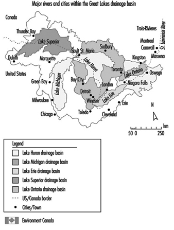
The Response
Since the 1950s, both countries have put in place domestic and bilateral programmes to address gross pollution problems and also to respond to more subtle water quality concerns. As a result of these actions, Great Lakes waters are visibly cleaner than they were at mid-century, loadings of heavy metals and organic chemicals have decreased and contaminant levels in fish and aquatic birds have gone down significantly. The successes of Canada–United States actions to restore and protect the Great Lakes provide a model for bilateral cooperation on resource management, but challenges remain.
The Case Study in Perspective
The threats posed by persistent toxic substances, however, are long term in nature and their management requires a multimedia, comprehensive at-source approach. To achieve a long-term goal of virtual elimination of persistent toxic substances from the Great Lakes, environmental authorities, industries and other stakeholders in the basin were challenged to develop new approaches and programmes. The purpose of this case study report is to provide a brief summary of Canadian pollution control programmes and the progress achieved by 1995, and to outline initiatives for managing persistent toxics in the Great Lakes. Similar US initiatives and programmes are not discussed herein. Interested readers should contact the Great Lakes National Program Office of the US Environmental Protection Agency in Chicago for information on federal and state programmes for protecting the Great Lakes.
1970s–1980s
A significant problem acknowledged to be affecting Lake Erie in the 1960s was nutrient enrichment or eutrophication. The identified need for bilateral actions prompted Canada and the United States to sign the first Great Lakes Water Quality Agreement (GLWQA) in 1972. The Agreement outlined abatement goals for reducing phosphorus loadings primarily from laundry detergents and municipal sewage effluent. In response to this commitment Canada and Ontario enacted legislation and programmes for controlling point sources. Between 1972 and 1987, Canada and Ontario invested more than 2 billion dollars in sewage treatment plant construction and upgrading in the Great Lakes basin.
Figure 2. Progress on industrial abatement
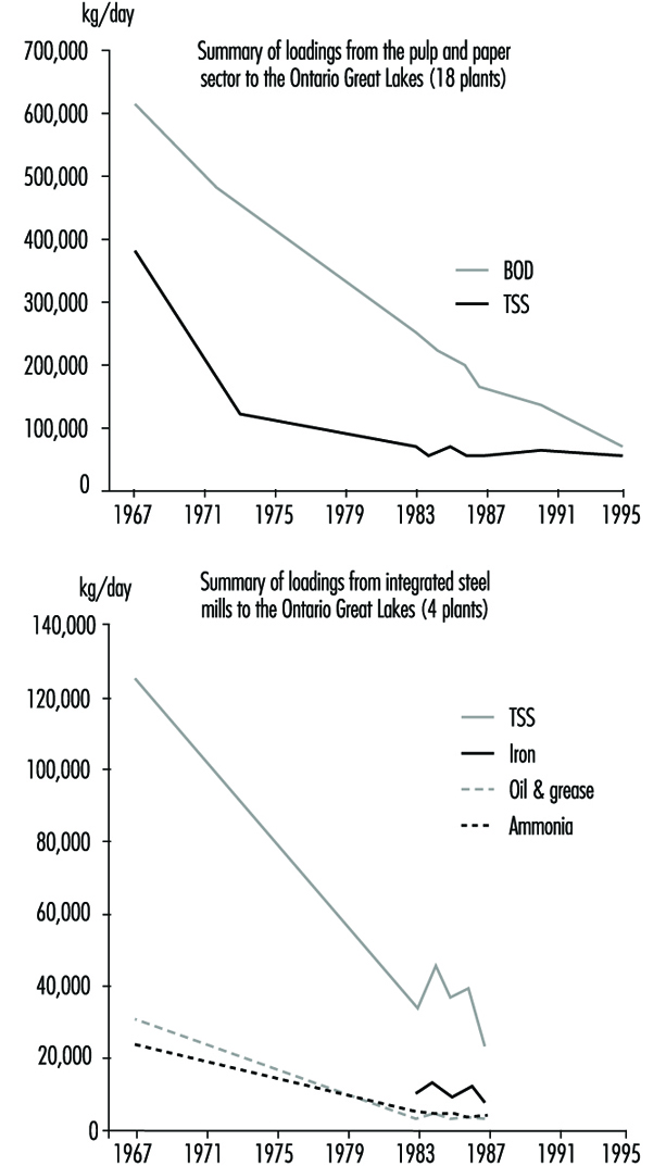
The 1972 GLWQA also identified the need to reduce releases of toxic chemicals into the lakes from industries and other sources such as spills. In Canada, the promulgation of federal effluent (end of pipe) regulations in the 1970s for conventional pollutants from major industrial sectors (pulp and paper, metal mining, petroleum refining and so on) provided a national baseline standard, while Ontario established similar effluent guidelines tailored for local needs including the Great Lakes. Actions by industries and municipalities to meet these federal and Ontario effluent requirements produced impressive results; for example, phosphorus loadings from point sources to Lake Erie were reduced by 70% between 1975 and 1989, and discharges of conventional pollutants from the seven Ontario petroleum refineries were cut by 90% since the early 1970s. Figure 2 shows similar loading reduction trends for the pulp and paper and the iron and steel sectors.
By the mid-1970s evidence of elevated concentrations of toxic chemicals in Great Lakes fish and wildlife, reproductive abnormalities in some fish-eating birds and population decline in a number of species implicated persistent bioaccumulative toxic substances, which became the new focus for the binational protection effort. Canada and the United States signed a second Great Lakes Water Quality Agreement in 1978, in which the two countries pledged to “restore and maintain the chemical, physical and biological integrity of the waters of the Great Lakes Ecosystem”. A key challenge was the policy “that the discharge of toxic substances in toxic amounts be prohibited and the discharge of any or all persistent toxic substances be virtually eliminated”. The call for virtual elimination was necessary, as persistent toxic chemicals may concentrate and accumulate in the food chain, causing severe and irreversible damages to the ecosystem, whereas chemicals which are not persistent needed to be kept below levels which cause immediate harm.
In addition to tighter controls on point sources, Canada and Ontario developed and/or strengthened controls on pesticides, commercial chemicals, hazardous wastes and non-point sources of pollution such as dump sites and incinerators. Government initiatives became more multimedia oriented, and the concept of “cradle to grave” or “responsible care” for chemicals became the new environmental management philosophy for government and industries alike. A number of persistent toxic pesticides were banned under the federal Pest Control Products Act (DDT, Aldrin, Mirex, Toxaphene, Chlordane) and the Environmental Contaminants Act was used to (1) prohibit commercial, manufacturing and processing uses of persistent toxics (CFC, PPB, PCB, PPT, Mirex, lead) and (2) to limit chemical releases from specific industrial operations (mercury, vinyl chloride, asbestos).
By the early 1980s, results from these programmes and measures and similar American efforts started producing evidence of a rebound. Contaminant levels in Great Lakes sediments, fish and wildlife were on the decline, and noted environmental improvements included the return of bald eagles to the Canadian shore of Lake Erie, a 200-fold increase in cormorant population, a resurgence in osprey on Georgian Bay and the re-establishment in the Toronto Harbour area of common terns - all have been affected by levels of persistent toxic substances in the past, and their recovery illustrates the success of this approach to date.
Figure 3. Mirex in herring gull eggs
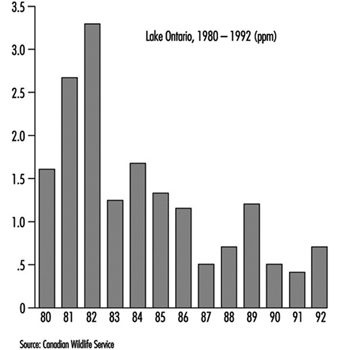
The trend toward reduced concentrations for some of the persistent toxic substances in fish, wildlife and sediments levelled off by the mid-1980s (see Mirex in herring gull eggs in figure 3). It was concluded by scientists that:
- While the water pollution and contaminants control programmes in place were helpful, they were not enough to bring about further reductions in contaminant concentrations.
- Additional measures were required for non-point sources of persistent toxics including contaminated sediments, long range atmospheric input of pollutants, abandoned dump sites and so on.
- Some pollutants can persist in the ecosystem at minute concentrations and can bioaccumulate in the food chain for a long time.
- The most efficient and effective approach for dealing with persistent toxics is to prevent or eliminate their generation at source rather than virtually eliminate their release.
It was generally agreed that achieving virtual elimination in the environment through the application of zero-discharge philosophy to sources and the ecosystem approach to Great Lakes water quality management needed to be further strengthened and promoted.
To reaffirm their commitment to the virtual elimination goal for persistent toxic substances, Canada and the United States amended the 1978 Agreement through a protocol in November 1987 (United States and Canada 1987). The protocol designated areas of concern where beneficial uses have been impaired around the Great Lakes, and required the development and implementation of remedial action plans (RAPs) for both point and non-point sources in the designated areas. The protocol also stipulated lakewide management plans (LAMPs) to be used as the main framework for resolving whole-lake impairment of beneficial uses and for coordinating control of persistent toxic substances impacting each of the Great Lakes. Furthermore, the protocol included new annexes for establishing programmes and measures for airborne sources, contaminated sediments and dump sites, spills and control of exotic species.
1990s
Following the signing of the 1987 protocol, the goal of virtual elimination was strongly promoted by environmental interest groups on both sides of the Great Lakes as concerns about the threat of persistent toxics increased. The International Joint Commission (IJC), the binational advisory body created under the 1909 Boundary Waters Treaty, also strongly advocated the virtual elimination approach. An IJC binational task force recommended a strategy for Virtual Elimination in 1993 (see figure 4). By the mid-1990s, the IJC and the parties are attempting to define a process for implementing this strategy, including considerations for socioeconomic impacts.
Figure 4. Decision-making process for virtual elimination of persistent toxic substances from the Great Lakes
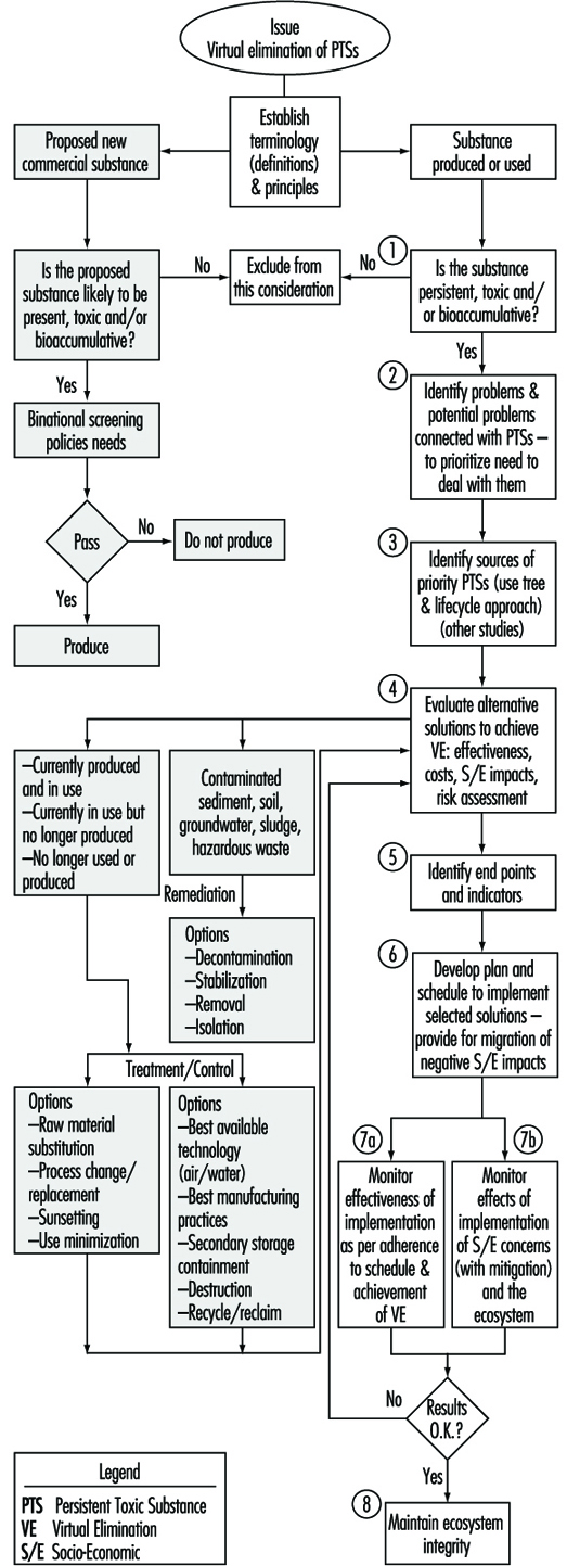
The governments of Canada and Ontario responded in a number of ways to control or reduce the release of persistent toxics. The important programmes and initiatives are briefly summarized below.
Canadian Environmental Protection Act (CEPA)
In 1989, Environment Canada consolidated and streamlined its legal mandates into a single statute. CEPA provides the federal government with comprehensive powers (e.g., information gathering, regulations making, enforcement) over the entire life cycle of chemicals. Under CEPA, the New Substances Notification Regulations establish screening procedures for new chemicals so that persistent toxics that cannot be adequately controlled will be prohibited from being imported, manufactured or used in Canada. The first phase of the Priority Substances List (PSL I) assessment programme was completed in 1994; 25 of the 44 substances assessed were found to be toxic under the definition of CEPA, and the development of management strategies for these toxic chemicals was initiated under a Strategic Options Process (SOP); an additional 56 priority substances will be nominated and assessed in phase II of the PSL programme by the year 2000. The National Pollutant Release Inventory (NPRI) was implemented in 1994 to mandate industrial and other facilities that meet the reporting criteria to annually report their releases to air, water and land, and their transfers in waste, of 178 specified substances. The inventory, modelled on the Toxic Release Inventory (TRI) in the United States, provides an important database for prioritizing pollution prevention and abatement programmes.
Canada-Ontario Agreement (COA)
In 1994, Canada and Ontario set out a strategic framework for coordinated action to restore, protect and conserve the Great Lakes ecosystem with a key focus on reducing the use, generation or release of 13 Tier I persistent toxic substances by the year 2000 (Canada and Ontario 1994). COA also targets an additional list of 26 priority toxics (Tier II) for significant reductions. Specifically for Tier I substances, COA will: (1) confirm zero discharge of five banned pesticides (Aldrin, DDT, Chlordane, Mirex, Toxaphene); (2) seek to decommission 90% of high-level PCBs, destroy 50% now in storage and accelerate destruction of low-level PCBs in storage; and (3) seek 90% reduction in the release of the remaining seven Tier I substances (benzo(a)pyrene, hexachlorobenzene, alkyl-lead, octachlorostyrene, PCDD (dioxins) PCDF (furans) and mercury).
The COA approach is to seek quantitative reductions wherever feasible, and sources are challenged to apply pollution prevention and other means to meet the COA targets. Fourteen projects have already been launched by federal Ontario staff to achieve reduction/elimination of Tiers I and II substances.
Toxic Substances Management Policy
In recognition of the need for a preventive and precautionary approach, Environment Canada announced in June 1995 a national Toxic Substances Management Policy as the framework for efficient management of toxic substances in Canada (Environment Canada 1995a). The policy adopts a two-track approach (see figure 5) that recognizes management actions must be tailored to the characteristics of chemicals; that is:
- to virtually eliminate from the environment substances that are predominantly anthropogenic, persistent, bioaccumulative and toxic (Track I)
- to implement full life cycle (cradle-to-grave) management of all other substances of concern (Track II).
Figure 5. Selection of management objectives under the Toxic Substances Management Policy
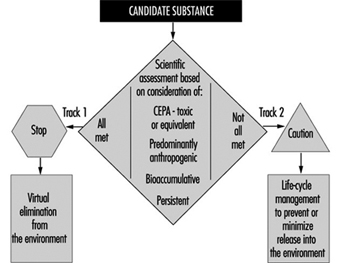
A set of scientifically based criteria (Environment Canada 1995b) (see table 1) will be used to categorize substances of concern into the two tracks. If a substance identified for either track is not adequately controlled under existing programmes, additional measures will be identified under the multi-stakeholder Strategic Options Process. The policy is consistent with the Great Lakes Water Quality Agreement and will direct and frame a number of domestic programmes by defining their ultimate environmental objective, but the means and pace of achieving the ultimate objective will vary by chemical and source. Further, Canada’s position on persistent toxics will also be framed by this policy in international discussions.
Table 1. Criteria for the selection of substances for Track 1 toxic substances management policy
|
Persistence |
Bioaccumulation |
Toxicity |
Predominantly Anthropogenic |
|
|
Medium |
Half-life |
|||
|
Air |
≥2 days |
BAF≥5,000 |
CEPA-toxic |
Concentration |
Chlorine Action Plan
A comprehensive approach to managing chlorinated substances within the context of the Toxic Substances Management Policy was announced in October 1994 by Environment Canada (Environment Canada 1994). The approach will be to prune the chlorine-use tree with a five-part action plan that will (1) target action on critical uses and products, (2) improve scientific understanding of chlorine and its impact on health and the environment, (3) detail socioeconomic implications, (4) improve public access to information and (5) promote international actions on chlorinated substances. Chlorine use has already decreased in Canada in recent years, for example by 45% in the pulp and paper sector since 1988. Implementation of the Chlorine Action Plan will accelerate this reduction trend.
Great Lakes Pollution Prevention Initiative
A strong pollution prevention programme has been put in place for the Great Lakes basin. Since March 1991, Environment Canada and the Ontario Ministry of the Environment and Energy have been working together with industries and other stakeholders to develop and implement pollution prevention projects, in contrast to waste treatment or reducing pollution after its generation. In 1995/96, more than 50 projects will cover commercial chemicals, hazardous waste management, federal facilities, industries, municipalities and the Lake Superior basin. Figure 6 provides an overview of these projects, which fall into two main categories: programme integration or voluntary agreements. The figure also shows programme linkages with other programmes discussed earlier (NPRI, RAP, LAMP) and a number of institutions that work with Environment Canada closely on green technologies and clean processes, as well as on training, information and communications. Pollution prevention projects can produce impressive results, as evidenced by the Automotive Manufacturers, who have undertaken 15 pilot projects recently, thereby reducing or eliminating 2.24 million kilograms of targeted substances from the manufacture of automobiles at the Ontario facilities of Chrysler, Ford and General Motors.
Figure 6. Great Lakes pollution prevention

Accelerated Reduction/Elimination of Toxics (ARET)
ARET is a cooperative multi-stakeholder initiative launched in 1994 that seeks the eventual elimination of 14 priority toxics with an interim target (by the year 2000) of a 90% reduction/elimination and reduced emission (50%) of 87 less harmful toxic substances (ARET Secretariat 1995). As of 1995, more than 200 companies and government agencies are participating in this voluntary initiative. Together, they reduced emissions by 10,300 tonnes in comparison with the 1988 base year and are committed to an additional 8,500 tonnes reduction by the year 2000.
Binational and international strategies
In addition to the above domestic initiatives, Canada and the United States are currently developing a binational strategy to coordinate agency action and to establish shared goals for persistent toxics in the Great Lakes basin. Goals and objectives similar to the Canada-Ontario Agreement for the Tiers I and II substances and a similar US list will be adopted. Joint projects will be developed and implemented to facilitate information exchange and agency action on priority chemicals such as PCBs and mercury. By taking an aggressive approach to virtual elimination as outlined above, Canada will be able to assume a leadership role in promoting international action on persistent toxics. Canada hosted a United Nations conference in June 1995 in Vancouver to focus global dialogue on persistent organic pollutants (POP) and to explore pollution prevention approaches to reducing their emissions around the world. Canada also co-chairs the United Nations Economic Commission for Europe (UNECE) workgroup to develop a protocol for persistent organic pollutants under the Convention on Long Range Transboundary Air Pollution.
An Example—Dioxins and Furans
For more than a decade, polychlorinated dibenzo-dioxins and furans have been recognized as a group of persistent toxics of concern to the Canadian environment and the Great Lakes. Table 2 summarizes federal actions and the reductions in releases achieved to date, illustrating the mix of programmes and initiatives which has resulted in significant reductions of these toxics. In spite of these impressive results, dioxins and furans will remain priorities under the Toxic Substances Management Policy, the Chlorine Action Plan, the Canada Ontario Agreement and the binational strategy outlined above, because virtual elimination requires further reductions.
Table 2. Summary of reductions in releases of dioxin and furan in Canada
|
Sources of Emissions |
Reductions |
Reporting Period |
Canadian Government Initiatives |
|
Bleached kraft pulpmill effluents |
82% |
1989-94 |
CEPA defoamer, wood chip and |
|
2,4,5-T—pesticide |
100% |
1985 |
Banned from use under PCPA |
|
2,4-D—pesticide |
100% |
1987-90 |
Dioxin content and use heavily |
|
Pentachlorophenol |
|
|
|
|
PCBs |
23% |
1984-93 |
CCME PCB Action Plan |
|
Incineration |
|
|
|
CCME: Canadian Council of Environmental Ministers; CEPA: Canadian Environmental Protection Act; PCPA: Pest Control Products Act.
Summary
There has been a significant improvement in the water quality of the Great Lakes as a result of pollution control actions taken by governments and stakeholders in Canada and the United States since the early 1970s. This case study report provides a summary of the Canadian effort and successes in dealing with gross pollution and conventional pollutants. It also outlines the evolution of a new approach (the Toxic Substances Management Policy, the Chlorine Action Plan, pollution prevention, voluntary action, stakeholder consultations and so on) for dealing with the much more difficult problems with persistent toxic substances in the Great Lakes. Comprehensive programmes (COA, NPRI, SOP, PSL and so on) that are being put in place with the aim of achieving the virtual elimination goal are briefly described. Details of the Canadian approach are contained in the listed references.
More...
Cleaner Production Technologies
Prevention, Control and Remediation
Conventionally, there are three ways of addressing pollution: prevention, control and remediation. These form a hierarchy, in which the first priority or option is prevention, followed by control measures, with remediation as a poor third. Pollution abatement can refer to any means that lessens pollution, or a mitigation of pollution; in practice, it usually means control. Though the hierarchy of the three ideas is in terms of preference or priority, this is not always so in practice: there may be regulatory pressures to choose one path rather than another; one strategy may be less expensive than another, or remediation may be the most urgent - for example, in the event of a major spill or the hazardous dissemination of pollutants from a contaminated site.
Pollution prevention
Pollution prevention can be defined as a strategy or strategies which avoid the creation of pollutants in the first place. In Barry Commoner’s phrase, “If it’s not there, it can’t pollute.” Thus, if a chemical whose use results in pollution is eliminated, there will be “zero discharge” (or “zero emission”) of the pollutant. Zero discharge is more convincing if the chemical is not replaced by another chemical - an alternative or substitute - which results in a different pollutant.
One central strategy of pollution prevention is the banning, elimination or the phasing out (“sunsetting”) of specified chemicals or classes of chemical. (Alternatively, use-restrictions may be specified.) Such strategies are laid down in the form of laws or regulations by national governments, less often by international instruments (conventions or treaties) or by sub-national governments.
A second strategy is pollution reduction, again in the context of prevention rather than control. If the use of a chemical which results in pollution is reduced, then the result will almost always be less pollution. Pollution reduction strategies are exemplified in North America by toxics use reduction (TUR) programmes and in Europe by “clean technology programmes”.
Unlike bans and phase-outs, which usually apply to all (relevant) workplaces within a political jurisdiction, pollution reduction programmes apply to specific workplaces or classes of workplace. These are usually industrial manufacturing (including chemical manufacturing) workplaces over a certain size, in the first instance, though the principles of pollution reduction can be applied generally - for example, to mines, power plants, construction sites, offices, agriculture (in regard to chemical fertilizers and pesticides) and municipalities. At least two US states (Michigan and Vermont) have legislated TUR programmes for individual households which are also workplaces.
Pollution reduction can result in the elimination of specific chemicals, thus achieving the same aims as bans and phase-outs. Again, this would result in zero discharge of the pollutant concerned, but requirements to eliminate specific chemicals are not part of pollution reduction programmes; what is prescribed is a general programme with a flexible range of specified methods. A requirement to eliminate a specific chemical is an example of a “specification standard”. A requirement to institute a general programme is a “performance standard” because it allows flexibility in the mode of implementation, though a specific mandatory target (outcome) for a general programme would (confusingly) count as a specification standard. When they have to choose, businesses usually prefer performance to specification standards.
Pollution control
Pollution control measures cannot eliminate pollution; all they can do is to mitigate its effects on the environment. Control measures are instituted “at the end of the (waste) pipe”. The usefulness of control measures will depend on the pollutant and the industrial circumstance. The main methods of pollution control, in no particular order, are:
- the capture and subsequent storage of pollutants
- filtration, whereby airborne or waterborne pollutants are removed from the waste stream by physical methods such as meshes, filters and other permeable barriers (such as coke)
- precipitation, whereby the pollutant is chemically precipitated and then captured in its transformed state or captured by physical methods such as an electrostatic charge
- destruction - for example, incineration, or neutralization, whereby pollutants are transformed chemically or biologically into substances which are less harmful
- dilution, whereby the pollutant is diluted or flushed in order to lessen its effects on any one organism or on an ecosystem; or concentration to lessen the effect of disposal
- evaporation or dissolution - for example, dissolving a gas in water
- utilization - for example, transforming a pollutant into a potentially useful (though not necessarily less toxic) product (such as sulphur dioxide into sulphuric acid or using solid waste as hard core or road bed)
- out-of-process recycling (where the recycling is not an integral part of the production process)
- media-shift, whereby a waste-stream is diverted from one medium, such as air, soil or water, to another, on the rationale that the medium-shift makes the pollutant less harmful
- state-changes—a change to the solid, liquid or gaseous state on the rationale that the new state is less harmful.
Pollution remediation
Remediation is needed to the extent that pollution prevention and control fail. It is also very expensive, with the costs not always accruing to the polluter. The modes of remediation are:
The clean-up of contaminated sites
Clean-up has a common sense meaning, as when an employer is required to “clean up his act”, which can mean a large number of different things. Within environmental protection, clean-up is a technical term meaning a branch or a mode of remediation. Even within this restricted use of the term, clean-up can mean (1) the removal of pollutants from a contaminated site or (2) the rehabilitation of a site so that it is restored to its full use-potential. Again, clean-up sometimes refers to nothing more than the containment of pollutants within a site, area or body of water—for example, by capping, sealing or the construction of an impermeable floor.
To be successful, clean-up has to be 100% effective, with full protection for workers, bystanders and the general public. A further consideration is whether the clean-up materials, methods and technology do not create further hazards. Though it is desirable to use engineering controls to protect clean-up workers, there will almost always be a need for appropriate personal protective equipment. Normally, workers engaged in remediation are classified as hazardous-waste workers, though aspects of such work are undertaken by fire fighters and municipal workers, among others.
A large number of physical, chemical, biological and biotechnological agents and methods are used in the clean-up of contaminated sites.
Hazardous-waste treatment
Most treatment of hazardous (or toxic) waste now takes place in purpose-built facilities by hazardous-waste workers. From an environmental point of view, the test of effectiveness of a hazardous-waste facility is that it produces no outputs which are not inert or virtually inert, such as silica, insoluble inorganic compounds, insoluble and non-corrosive slags, gaseous nitrogen or carbon dioxide - though carbon dioxide is a “greenhouse gas” which causes climate change and is, thus, a further environmental detriment.
A further test is that the facility be energy efficient - that is, energy is not wasted - and as energy non-intensive as possible (i.e., the ratio of energy use to the volume of waste treated be as low as possible). A general rule of thumb (it is fortunately not a universal law) is that the more effective the pollution (or waste) abatement strategy, the more energy is consumed, which by sustainable development criteria is another detriment.
Even when the workers are properly protected, it is easy to see the drawbacks of hazardous-waste treatment as a mode of addressing pollution. Pollution prevention methods can be applied to the operation of the treatment process but they cannot be applied to the principal “input” - the waste to be treated. Hazardous-waste treatment facilities will usually require at least as much energy to treat the waste as was expended in its creation, and there will always be further waste as an output, however inert or non-toxic.
Spills and leaks
The same considerations will apply to chemical spills and leaks as to the clean-up of contaminated sites, with the further hazards caused by the urgency of the clean-up. Workers cleaning up spills and leaks are almost always emergency workers. Depending on the scale and the nature of the pollutant, leaks and spills can become major industrial accidents.
The Modes of Pollution Prevention
Definition and philosophy
The definition of pollution prevention may seem to be a trivial matter, but it is important because advocates of pollution prevention want, as a principle of policy, to see a single-minded and aggressive prevention strategy at the expense of control methods, and to avoid remediation. The more strictly pollution prevention is defined, they say, the more likely it is to succeed as a practical strategy. Conversely, the more widely employers are allowed to define the term, the more likely their activities are to result in a mix of the same old (failed) strategies. Employers sometimes reply that even toxic waste can have a market value, and control methods have their place, so pollution is really only potential pollution. Besides, zero discharge is impossible and leads only to false expectations and misguided strategies. Proponents of pollution prevention respond that unless we have zero discharge as an aim or practical ideal, pollution prevention will not succeed and environmental protection will not improve.
Most of the strict definitions of pollution prevention have, as a sole or central element, the avoidance of the use of chemicals which result in pollutants so that pollution is not created in the first place. Some of the most important definitional controversies concern recycling, which is dealt with in the context of pollution prevention below.
Objectives
One possible objective of pollution prevention is zero discharge of pollutants. This is sometimes referred to as “virtual elimination”, since even zero discharge cannot solve the problem of contaminants already in the environment. Zero discharge of pollutants is possible using pollution prevention methods (while control methods cannot achieve zero in theory and are even less effective in practice, usually owing to lax enforcement). For instance, we can envisage automobile production in which there is zero discharge of pollutants from the plant; other waste is recycled and the product (the car) consists of parts which are reusable or recyclable. Certainly, zero discharge of specific pollutants has been achieved - for example, by modifying the production process in wood pulp mills so that no dioxins or furans are discharged in the effluent. The aim of zero discharge has also been written into environmental laws and into the policies of bodies commissioned to abate pollution.
In practice, zero discharge often gives way to target reductions - for example, a 50% reduction in pollution emissions by such-and-such a year. These targets or interim targets are usually in the form of “challenges” or aims by which to measure the success of the pollution prevention programme. They are rarely the product of a feasibility analysis or calculation, and there are invariably no penalties attached to failure to attain the target. Nor are they measured with any precision.
Reductions would have to be measured (as opposed to estimated) by variations on the formula:
Pollution (P) = Toxicity of the pollutant (T) × Volume (V) of the discharges
or:
P = T x V x E (exposure potential).
This is very difficult in theory and expensive in practice, though it could be done in principle by utilizing hazard assessment techniques (see below). The whole issue suggests that resources would be better allocated elsewhere - for example, in ensuring that proper pollution prevention plans are produced.
In regard to chemical pesticides, the objective of use-reduction can be achieved by the methods of integrated pest management (IPM), though this term, too, is capable of a wide or a strict definition.
Methods
The main methods of pollution prevention are:
- The elimination or phasing out of specific hazardous chemicals
- Input substitution - replacing a toxic or hazardous substance with a non-toxic or less hazardous substance or with a non-toxic process. Examples are the substitution of water-based for synthetic organic dyes in the printing industry; water - or citrus-based solvents for organic solvents; and, in some applications, the substitution of vegetable for mineral oils. Examples of non-chemical substitution include the substitution of pellet blasting technology for the use of fluid chemical paint strippers; the use of high-pressure hot water systems instead of caustic cleaning; and the substitution of kiln-drying for the use of pentachlophenols (PCPs) in the lumber industry.
In all cases, it is necessary to perform a substitution analysis to ensure that substitutes are genuinely less hazardous than what they replace. This is at least a matter of organized common sense, and at best the application of hazard assessment techniques (see below) to the chemical and its proposed substitute.
- Product reformulation - substituting for an existing end-product an end-product which is non-toxic or less toxic upon use, release or disposal
Whereas input substitution refers to the raw materials and adjuncts at the “front end” of the production process, product reformulation approaches the issue from the final product end of the production cycle.
General programmes to produce products which are more environmentally benign are examples of “economic conversion”. Examples of particular measures in the area of product reformulation include the production of rechargeable batteries instead of throw-away types and the use of water-based product coatings instead of those based on organic solvents and the like.
Again, substitution analysis will be necessary to ensure that the net environmental benefit is greater for the reformulated products that it is for the originals.
- Production unit redesign modernization or modification, which results in less chemical use or in the use of less toxic substances.
- Improved operation and maintenance of the production unit and production methods, including better housekeeping, more efficient production quality control, and process inspections.
Examples are spill prevention measures; the use of spill-proof containers; leak prevention; and floating lids for solvent tanks.
- Using less and reusing more. For instance, some degreasing operations take place too frequently on a single item. In other cases, chemicals can be used more sparingly in each operation. De-icing fluids can sometimes be reused, a case of “extended use”.
- Closed-loop methods and in-process recycling. Strictly speaking, a closed-loop process is one in which there are no emissions into the workplace or into the outside environment, not even waste water into surface water or carbon dioxide into the atmosphere. There are only inputs, finished products, and inert or non-toxic wastes. In practice, closed-loop methods eliminate some, but not all, hazardous releases. To the extent that this is achieved, it will count as a case of in-process recycling (see below).
Recycling
Any definition of pollution prevention is likely to result in a number of “grey areas” in which it is not easy to distinguish prevention measures from emission controls. For instance, to qualify as a prevention method, a phase of a production process may have to be “an integral part of the production unit”, but how far away the phase has to be from the periphery of the production process in order to qualify as a prevention measure is not always clear. Some processes may be so remote from the heart of an operation that they look more like an “add on” process and, thus, more like an “end of pipe” control measure than a prevention method. Again, there are unclear cases like a waste pipe that provides the feedstock for a neighbouring plant: taken together, the two plants provide a kind of closed loop; but the “upstream” plant still produces effluent and, thus, fails the prevention test.
Similarly with recycling. Conventionally, there are three types of recycling:
- in-process recycling - for example, when dry-cleaning solvent is filtered, cleaned and dried, then reused within a single process
- out-of-process but on-site, as when pesticide production waste is cleaned and then reused as the so-called inert base in a new production run
- out-of-process and off-site.
Of these, the third is usually ruled out as not qualifying as pollution prevention: the more remote the recycling site, the less of a guarantee that the recycled product is actually reused. There are also hazards in the transporting of waste to be recycled, and the financial uncertainty that the waste will have a continuous market value. Similar, though less acute, considerations apply to out-of-process but on-site recycling: there is always a possibility that the waste will not actually be recycled or, if recycled, not actually reused.
In the initial pollution prevention strategies of the 1980s, on-site but out-of-process recycling was ruled out as not being a genuine pollution prevention measure. There was a fear that an effective pollution prevention programme would be compromised or diluted by too great an emphasis on recycling. In the mid-1990s, some policy-makers are prepared to entertain on-site, out-of-process recycling as a legitimate pollution prevention method. One reason is that there are genuine “grey areas” between prevention and control. Another reason is that some on-site recycling really does do what it is supposed to do, even though it may not technically qualify as pollution prevention. A third reason is business pressure: employers see no reason why techniques should be ruled out it they serve the purposes of a pollution prevention programme.
Pollution prevention planning
Planning is an essential part of pollution prevention methodology, not least because the gains in both industrial efficiency and environmental protection are likely to be in the longer term (not immediate), reflecting the sort of planning that goes into product design and marketing. The production of periodic pollution prevention plans is the most usual way of realizing pollution prevention planning. There is no single model for such plans. One proposal envisages:
- aims and objectives
- chemical inventories and estimates of discharges into the environment
- pollution prevention methods used and methods proposed
- responsibilities and action in the event of the plan not being fulfilled or realized.
Another proposal envisages:
- a review of production processes
- identification of pollution prevention opportunities
- a ranking of the opportunities and a schedule for the implementation of the selected options
- measures of the success of the plan after the implementation period.
The status of such plans varies widely. Some are voluntary, though they can be spelled out in law as a (voluntary) code of practice. Others are mandatory in that they are required (1) to be kept on-site for inspection or (2) submitted to a regulatory authority on completion or (3) submitted to a regulatory authority for some form of scrutiny or approval. There are also variations, such as requiring a plan in the event that a “voluntary” plan is, in some way, inadequate or ineffective.
The degree to which mandatory plans are prescriptive also varies - for example, in regard to penalties and sanctions. Few authorities have the power to require specific changes in the content of pollution prevention plans; almost all have the power to require changes in the plan in the event that the formal requirements have not been met - for example, if some plan headings have not been addressed. There are virtually no examples of penalties or sanctions in the event that the substantive requirements of a plan have not been met. In other words, legal requirements for pollution prevention planning are far from traditional.
Issues surrounding the production of pollution prevention plans concern the degree of confidentiality of the plans: in some cases, only a summary becomes public, while in other cases, plans are released only when the producer fails in some way to comply with the law. In almost no cases do the requirements for pollution prevention planning override existing provisions regarding the trade secrecy or the business confidentiality of inputs, processes or the ingredients of products. In a few cases, community environmental groups have access to the planning process, but there are virtually no cases of this being required by law, nor are the legal rights of workers to participate in the production of plans widespread.
Legislation
In the Canadian provinces of British Columbia and Ontario, pollution prevention measures are “voluntary”; their effectiveness depends on “moral suasion” on the part of governments and environmentalists. In the United States, about half (26) of the states have some form of legislation, while in Europe, several northern countries have legislated clean technology programmes. There is quite a wide variety in both the content and the effectiveness of such legislation. Some laws define pollution prevention strictly; others define it widely or loosely and cover a wide variety of environmental protection activities concerning pollution and waste, not just pollution prevention. The New Jersey law is highly prescriptive; those of the Commonwealth of Massachusetts and the States of Minnesota and Oregon involve a high degree of government scrutiny and assistance; that of Alaska is little more than a statement of the government’s intentions.
Health, safety and employment
Pollution prevention is of central concern to occupational health: if the use of toxic substances decreases, there will almost always be a corresponding decrease in worker exposure to toxic substances and, thus, in industrial diseases. This is a prime case of prevention “at the source” of the hazard and, in many cases, the elimination of hazards by “engineering controls”
(i.e., methods), the first and best line of defence against chemical hazards. However, such preventive measures are different from one traditional strategy, which is the “total isolation” or the “total enclosure” of a chemical process. While total enclosure is highly useful and highly desirable, it does not count as a pollution prevention method since it controls, rather that reduces intrinsically, an existing hazard.
The pollutants which pose hazards to workers, communities and the physical environment alike, have usually been addressed primarily because of their impact on human communities (environmental health). Though the greatest exposures are often received by workers within a workplace (workplace pollution), this has not, so far, been the prime focus of pollution prevention measures. The Massachusetts legislation, for instance, aims to reduce the risks to the health of workers, consumers and the environment without shifting the risks between workers, consumers and parts of the environment (New Jersey is similar). But there was no attempt to focus on workplace pollution as a major detriment, nor was there a requirement to accord a primacy to the chief human exposures to hazards - often the workers. Nor is there any requirement to train workers in the discipline of pollution prevention.
There are several reasons for this. The first is that pollution prevention is a new discipline in the context of a general, traditional failure to see environmental protection as a function of processes utilized and adopted within workplaces. A second reason is that worker-management co-determination in the area of environmental protection is not well advanced. Workers in many countries have legal rights, for instance, to joint workplace health and safety committees; to refuse unsafe or unhealthy work; to health and safety information; and to training in health and safety issues and procedures. But there are few legal rights in the parallel and often overlapping area of environmental protection, such as the right to joint union-management environment committees; the right of employees to “blow the whistle” (go public) on an employer’s anti-environmental practices; the right to refuse to pollute or to degrade the outside environment; the right to environmental information; and the right to participate in workplace environmental audits (see below).
The impacts of pollution prevention planning on employment are hard to gauge. The explicit aim of pollution prevention initiatives is often to increase industrial efficiency and environmental protection at the same time and by the same set of measures. When this happens, the usual effect is to decrease overall employment within any given workplace (because of technological innovation) but to increase the skills required and then to increase job security (because there is planning for a longer-term future). To the extent that the use of raw materials and adjuncts is reduced, there will be decreased chemical manufacturing employment, though this is likely to be offset by the implied transition of feedstock to speciality chemicals and by the development of alternatives and substitutes.
There is one aspect of employment which pollution prevention planning cannot address. Pollution emissions from a single facility may decrease but to the extent that there is an industrial strategy to create wealth and value-added employment, an increase in the number of production facilities (however “clean”) will tend to nullify the environmental protection gains already achieved. The most notorious failing in environmental protection measures - that pollution emission reductions and controls are nullified by an increase in the number of sources - applies, unfortunately, to pollution prevention as well as to any other form of intervention. Ecosystems, according to one respected theory, have a “carrying capacity”, and that limit can be reached equally by a small number of highly polluting or “dirty” sources or by a correspondingly large number of clean ones.
Workplace environmental audits
Pollution prevention planning can form part of or be accommodated in a workplace environmental audit. Though there are many versions of such audits, they are likely to be in the form of a “site audit” or “production audit”, in which the whole production cycle is subjected to both an environmental and a financial analysis.
There are roughly three areas of sustainable development and environmental protection which can be covered in a workplace audit:
- the conservation of natural resource inputs - for example, minerals, water and wood products
- energy use, which may also include consideration of energy sources, energy efficiency, energy intensiveness and energy conservation
- pollution prevention, control and remediation.
To the extent that pollution prevention is successful, there will be a corresponding decrease in the importance of control and remediation measures; pollution prevention measures can form a major part of a workplace environmental audit.
Traditionally, businesses were able to “externalize” environmental detriments through such means as the profligate use of water or unloading their wastes onto the outside community and the environment. This has led to demands for taxes on the “front end” such as water use or on “outputs” such as environmentally unfriendly products or on wastes (“pollution taxes”).
In this way, costs to business are “internalized”. However, it has proved difficult to put the right price on the inputs and on the detriments - for example, the cost to communities and the environment of wastes. Nor is it clear that pollution taxes reduce pollution in proportion to the amounts levied; taxes may well “internalize” costs, but they otherwise only add to the cost of doing business.
The advantage of environmental auditing is that the audit can make economic sense without having to “cost” externalities. For instance, the “value” of waste can be calculated in terms of resource input loss and energy “non-utilization” (inefficiency) - in other words, of the difference in value between resources and energy on one side and the value of the product on the other. Unfortunately, the financial side of pollution prevention planning and its part in workplace environmental audits is not well advanced.
Hazard assessment
Some pollution prevention schemes work without any hazard evaluation - that is, without criteria to decide whether a plant or facility is more or less environmentally benign as a result of pollution prevention measures. Such schemes may rely on a list of chemicals which are objects of concern or which define the scope of the pollution prevention programme. But the list does not grade chemicals as to their relative hazardousness, nor is there a guarantee that a chemical substitute not on the list is, in fact, less hazardous than a listed chemical. Common sense, not scientific analysis, tells us how to go about implementing a pollution prevention programme.
Other schemes rest on criteria for assessing hazardousness, that is, on hazard assessment systems. They work, essentially, by laying down a number of environmental parameters, such as persistence and bioaccumulation in the environment, and a number of human health parameters which serve as measures of toxicity - for example, acute toxicity, carcinogenicity, mutagenicity, reproductive toxicity and so on.
There is then a weighted scoring system and a decision procedure for scoring those parameters on which there is inadequate information on the chemicals to be scored. Relevant chemicals are then scored and ranked, then (often) assembled in groups in descending order of hazardousness.
Though such schemes are sometimes devised with a specific purpose in mind - for example, for assessing priorities for control measures or for elimination (banning) - their essential use is as an abstract scheme which can be used for a large variety of environmental protection measures, including pollution prevention. For instance, the top group of scored chemicals could be the prime candidates for a mandatory pollution prevention programme, or they could be candidates for phasing-out or substitution. In other words, such schemes do not tell us how much we should reduce environmental health hazards; they tell us only that any measures we take should be informed by the hazard assessment scheme.
For instance, if we have to make decisions about substituting a less hazardous chemical for a more dangerous one, we can use the scheme to tell us whether, prima facie, the substitution decision is a good one: we run both chemicals through the scheme to determine whether there is a wide or merely a narrow gap between them regarding their hazardousness.
There are two sorts of considerations which rarely fall within the scope of hazard assessment schemes. The first is exposure data, or the potential for human exposure to the chemical. The latter is difficult to calculate, and, arguably, it distorts the “intrinsic hazard” of the chemicals concerned. For instance, a chemical could be accorded an artificially low priority on the grounds that its exposure potential is low; though it may, in fact, be highly toxic and relatively easy to deal with.
The second sort of consideration is the socioeconomic impact of eliminating or reducing the use of the chemical concerned. While we can start to make substitution decisions on the basis of the hazard analysis, we would have to make a further and distinct socioeconomic analysis and consider, for example, the social utility of the product associated with the chemical use (which may, e.g., be a useful drug), and we would also have to consider the impact on workers and their communities. The reason for keeping such analysis separate is that it is impossible to score the results of a socioeconomic analysis in the same way that the intrinsic hazards of chemicals are scored. There are two entirely distinct sets of values with different rationales.
However, hazard assessment schemes are crucial in assessing the success of pollution prevention programmes. (They are also relatively new, both in their impact and their utility.) For instance, it is possible to apply them without reference to risk assessments, risk analysis and (with reservations) without reference to cost-benefit analysis. An earlier approach to pollution was to first do a risk assessment and only then decide what sort of action, and how much, was necessary to reduce the risk to an “acceptable” level. The results were rarely dramatic. Hazard assessment, on the other hand, can be utilized very quickly and in such a way that it does not delay or compromise the effectiveness of a pollution prevention programme. Pollution prevention is, above all, a pragmatic programme capable of constantly and speedily addressing pollution issues as they arise and before they arise. It is arguable that traditional control measures have reached their limit and only the implementation of comprehensive pollution prevention programmes will be capable of addressing the next phase of environmental protection in a practical and effective way.
" DISCLAIMER: The ILO does not take responsibility for content presented on this web portal that is presented in any language other than English, which is the language used for the initial production and peer-review of original content. Certain statistics have not been updated since the production of the 4th edition of the Encyclopaedia (1998)."