- You are here:
-
Home

-
Part XVII. Services and Trade
-
Health Care Facilities and Services
- Healthcare Workers and Infectious Diseases
Regulations, Recommendations, Guidelines and Standards
Criteria for Establishment
The setting of specific guides and standards for indoor air is the product of proactive policies in this field on the part of the bodies responsible for their establishment and for maintaining the quality of indoor air at acceptable levels. In practice, the tasks are divided and shared among many entities responsible for controlling pollution, maintaining health, ensuring the safety of products, watching over occupational hygiene and regulating building and construction.
The establishment of a regulation is intended to limit or reduce the levels of pollution in indoor air. This goal can be achieved by controlling the existing sources of pollution, diluting indoor air with outside air and checking the quality of available air. This requires the establishment of specific maximum limits for the pollutants found in indoor air.
The concentration of any given pollutant in indoor air follows a model of balanced mass expressed in the following equation:

where:
Ci = the concentration of the pollutant in indoor air (mg/m3);
Q = the emission rate (mg/h);
V = the volume of indoor space (m3);
Co = the concentration of the pollutant in outdoor air (mg/m3);
n = the ventilation rate per hour;
a = the pollutant decay rate per hour.
It is generally observed that—in static conditions—the concentration of pollutants present will depend in part on the amount of the compound released into the air from the source of contamination and its concentration in outdoor air, and on the different mechanisms by which the pollutant is removed. The elimination mechanisms include the dilution of the pollutant and its “disappearance” with time. All regulations, recommendations, guidelines and standards that may be set in order to reduce pollution must take stock of these possibilities.
Control of the Sources of Pollution
One of the most effective ways to reduce the levels of concentration of a pollutant in indoor air is to control the sources of contamination within the building. This includes the materials used for construction and decoration, the activities within the building and the occupants themselves.
If it is deemed necessary to regulate emissions that are due to the construction materials used, there are standards that limit directly the content in these materials of compounds for which harmful effects to health have been demonstrated. Some of these compounds are considered carcinogenic, like formaldehyde, benzene, some pesticides, asbestos, fibreglass and others. Another avenue is to regulate emissions by the establishment of emission standards.
This possibility presents many practical difficulties, chief among them being the lack of agreement on how to go about measuring these emissions, a lack of knowledge about their effects on the health and comfort of the occupants of the building, and the inherent difficulties of identifying and quantifying the hundreds of compounds emitted by the materials in question. One way to go about establishing emission standards is to start out from an acceptable level of concentration of the pollutant and to calculate a rate of emission that takes into account the environmental conditions—temperature, relative humidity, air exchange rate, loading factor and so forth—that are representative of the way in which the product is actually used. The main criticism levelled against this methodology is that more than one product may generate the same polluting compound. Emission standards are obtained from readings taken in controlled atmospheres where conditions are perfectly defined. There are published guides for Europe (COST 613 1989 and 1991) and for the United States (ASTM 1989). The criticisms usually directed against them are based on: (1) the fact that it is difficult to get comparative data and (2) the problems that surface when an indoor space has intermittent sources of pollution.
As for the activities that may take place in a building, the greatest focus is placed on building maintenance. In these activities the control can be established in the form of regulations about the performance of certain duties—like recommendations relating to the application of pesticides or the reduction of exposure to lead or asbestos when a building is being renovated or demolished.
Because tobacco smoke—attributable to the occupants of a building—is so often a cause of indoor air pollution, it deserves separate treatment. Many countries have laws, at the state level, that prohibit smoking in certain types of public space such as restaurants and theatres, but other arrangements are very common whereby smoking is permitted in certain specially designated parts of a given building.
When the use of certain products or materials is prohibited, these prohibitions are made based on their alleged detrimental health effects, which are more or less well documented for levels normally present in indoor air. Another difficulty that arises is that often there is not enough information or knowledge about the properties of the products that could be used in their stead.
Elimination of the Pollutant
There are times when it is not possible to avoid the emissions of certain sources of pollution, as is the case, for example, when the emissions are due to the occupants of the building. These emissions include carbon dioxide and bioeffluents, the presence of materials with properties that are not controlled in any way, or the carrying out of everyday tasks. In these cases one way to reduce the levels of contamination is with ventilation systems and other means used to clean indoor air.
Ventilation is one of the options most heavily relied on to reduce the concentration of pollutants in indoor spaces. However, the need to also save energy requires that the intake of outside air to renew indoor air be as sparing as possible. There are standards in this regard that specify minimum ventilation rates, based on the renewal of the volume of indoor air per hour with outdoor air, or that set a minimum contribution of air per occupant or unit of space, or that take into account the concentration of carbon dioxide considering the differences between spaces with smokers and without smokers. In the case of buildings with natural ventilation, minimum requirements have also been set for different parts of a building, such as windows.
Among the references most often cited by a majority of the existing standards, both national and international—even though it is not legally binding—are the norms published by the American Society of Heating, Refrigerating and Air Conditioning Engineers (ASHRAE). They were formulated to aid air-conditioning professionals in the design of their installations. In ASHRAE Standard 62-1989 (ASHRAE 1989), the minimum amounts of air needed to ventilate a building are specified, as well as the acceptable quality of indoor air required for its occupants in order to prevent adverse health effects. For carbon dioxide (a compound most authors do not consider a pollutant given its human origin, but that is used as an indicator of the quality of indoor air in order to establish the proper functioning of ventilation systems) this standard recommends a limit 1,000 ppm in order to satisfy criteria of comfort (odour). This standard also specifies the quality of outdoor air required for the renewal of indoor air.
In cases where the source of contamination—be it interior or exterior—is not easy to control and where equipment must be used to eliminate it from the environment, there are standards to guarantee their efficacy, such as those that state specific methods to check the performance of a certain type of filter.
Extrapolation from Standards of Occupational Hygiene to Standards of Indoor Air Quality
It is possible to establish different types of reference value that are applicable to indoor air as a function of the type of population that needs to be protected. These values can be based on quality standards for ambient air, on specific values for given pollutants (like carbon dioxide, carbon monoxide, formaldehyde, volatile organic compounds, radon and so on), or they can be based on standards usually employed in occupational hygiene. The latter are values formulated exclusively for applications in industrial environments. They are designed, first of all, to protect workers from the acute effects of pollutants—like irritation of mucous membranes or of the upper respiratory tract—or to prevent poisoning with systemic effects. Because of this possibility, many authors, when they are dealing with indoor environment, use as a reference the limit values of exposure for industrial environments established by the American Conference of Governmental Industrial Hygienists (ACGIH) of the United States. These limits are called threshold limit values (TLVs), and they include limit values for workdays of eight hours and work weeks of 40 hours.
Numerical ratios are applied in order to adapt TLVs to the conditions of the indoor environment of a building, and the values are commonly reduced by a factor of two, ten, or even one hundred, depending on the kind of health effects involved and the type of population affected. Reasons given for reducing the values of TLVs when they are applied to exposures of this kind include the fact that in non-industrial environments personnel are exposed simultaneously to low concentrations of several, normally unknown chemical substances which are capable of acting synergistically in a way that cannot be easily controlled. It is generally accepted, on the other hand, that in industrial environments the number of dangerous substances that need to be controlled is known, and is often limited, even though concentrations are usually much higher.
Moreover, in many countries, industrial situations are monitored in order to secure compliance with the established reference values, something that is not done in non-industrial environments. It is therefore possible that in non-industrial environments, the occasional use of some products can produce high concentrations of one or several compounds, without any environmental monitoring and with no way of revealing the levels of exposure that have occurred. On the other hand, the risks inherent in an industrial activity are known or should be known and, therefore, measures for their reduction or monitoring are in place. The affected workers are informed and have the means to reduce the risk and protect themselves. Moreover, workers in industry are usually adults in good health and in acceptable physical condition, while the population of indoor environments presents, in general, a wider range of health statuses. The normal work in an office, for example, may be done by people with physical limitations or people susceptible to allergic reactions who would be unable to work in certain industrial environments. An extreme case of this line of reasoning would apply to the use of a building as a family dwelling. Finally, as noted above, TLVs, just like other occupational standards, are based on exposures of eight hours a day, 40 hours a week. This represents less than one fourth of the time a person would be exposed if he or she remained continually in the same environment or were exposed to some substance for the entire 168 hours of a week. In addition, the reference values are based on studies that include weekly exposures and that take into account times of non-exposure (between exposures) of 16 hours a day and 64 hours on weekends, which makes it is very hard to make extrapolations on the strength of these data.
The conclusion most authors arrive at is that in order to use the standards for industrial hygiene for indoor air, the reference values must include a very ample margin of error. Therefore, the ASHRAE Standard 62-1989 suggests a concentration of one tenth of the TLV value recommended by the ACGIH for industrial environments for those chemical contaminants which do not have their own established reference values.
Regarding biological contaminants, technical criteria for their evaluation which could be applicable to industrial environments or indoor spaces do not exist, as is the case with the TLVs of the ACGIH for chemical contaminants. This could be due to the nature of biological contaminants, which exhibit a wide variability of characteristics that make it difficult to establish criteria for their evaluation that are generalized and validated for any given situation. These characteristics include the reproductive capacity of the organism in question, the fact that the same microbial species may have varying degrees of pathogenicity or the fact that alterations in environmental factors like temperature and humidity may have an effect upon their presence in any given environment. Nonetheless, in spite of these difficulties, the Bioaerosol Committee of the ACGIH has developed guidelines to evaluate these biological agents in indoor environments: Guidelines for the Assessment of Bioaerosols in the Indoor Environment (1989). The standard protocols that are recommended in these guidelines set sampling systems and strategies, analytical procedures, data interpretation and recommendations for corrective measures. They can be used when medical or clinical information points to the existence of illnesses like humidifier fever, hypersensitivity pneumonitis or allergies related to biological contaminants. These guidelines can be applied when sampling is needed in order to document the relative contribution of the sources of bioaerosols already identified or to validate a medical hypothesis. Sampling should be done in order to confirm potential sources, but routine sampling of air to detect bioaerosols is not recommended.
Existing Guidelines and Standards
Different international organizations such as the World Health Organization (WHO) and the International Council of Building Research (CIBC), private organizations such as ASHRAE and countries like the United States and Canada, among others, are establishing exposure guidelines and standards. For its part, the European Union (EU) through the European Parliament, has presented a resolution on the quality of air in indoor spaces. This resolution establishes the need for the European Commission to propose, as soon as possible, specific directives that include:
- a list of substances to be proscribed or regulated, both in the construction and in the maintenance of buildings
- quality standards that are applicable to the different types of indoor environments
- prescriptions for the consideration, construction, management and maintenance of air-conditioning and ventilation installations
- minimum standards for the maintenance of buildings that are open to the public.
Many chemical compounds have odours and irritating qualities at concentrations that, according to current knowledge, are not dangerous to the occupants of a building but that can be perceived by—and therefore annoy—a large number of people. The reference values in use today tend to cover this possibility.
Given the fact that the use of occupational hygiene standards is not recommended for the control of indoor air unless a correction is factored in, in many cases it is better to consult the reference values used as guidelines or standards for the quality of ambient air. The US Environmental Protection Agency (EPA) has set standards for ambient air intended to protect, with an adequate margin of safety, the health of the population in general (primary standards) and even its welfare (secondary standards) against any adverse effects that may be predicted due to a given pollutant. These reference values are, therefore, useful as a general guide to establish an acceptable standard of air quality for a given indoor space, and some standards like ASHRAE-92 use them as quality criteria for the renewal of air in a closed building. Table 1 shows the reference values for sulphur dioxide, carbon monoxide, nitrogen dioxide, ozone, lead and particulate matter.
Table 1. Standards of air quality established by the US Environmental Protection Agency
|
Average concentration |
|||
|
Pollutant |
μg/m3 |
ppm |
Time frame for exposures |
|
Sulphur dioxide |
80a |
0.03 |
1 year (arithmetic mean) |
|
365a |
0.14 |
24 hoursc |
|
|
1,300b |
0.5 |
3 hoursc |
|
|
Particulate matter |
150a,b |
— |
24 hoursd |
|
50a,b |
— |
1 yeard (arithmetic mean) |
|
|
Carbon monoxide |
10,000a |
9.0 |
8 hoursc |
|
40,000a |
35.0 |
1 hourc |
|
|
Ozone |
235a,b |
0.12 |
1 hour |
|
Nitrogen dioxide |
100a,b |
0.053 |
1 year (arithmetic mean) |
|
Lead |
1.5a,b |
— |
3 months |
a Primary standard. b Secondary standard. c Maximum value that should not be exceeded more than once a year. d Measured as particles of diameter ≤10 μm. Source: US Environmental Protection Agency. National Primary and Secondary Ambient Air Quality Standards. Code of Federal Regulations, Title 40, Part 50 (July 1990).
For its part, WHO has established guidelines intended to provide a baseline to protect public health from adverse effects due to air pollution and to eliminate or reduce to a minimum those air pollutants that are known or suspected of being dangerous for human health and welfare (WHO 1987). These guidelines do not make distinctions as to the type of exposure they are dealing with, and hence they cover exposures due to outdoor air as well as exposures that may occur in indoor spaces. Tables 2 and 3 show the values proposed by WHO (1987) for non-carcinogenic substances, as well as the differences between those that cause health effects and those that cause sensory discomfort.
Table 2. WHO guideline values for some substances in air based on known effects on human health other than cancer or odour annoyance.a
|
Pollutant |
Guideline value (time- |
Duration of exposure |
|
Organic compounds |
||
|
Carbon disulphide |
100 μg/m3 |
24 hours |
|
1,2-Dichloroethane |
0.7 μg/m3 |
24 hours |
|
Formaldehyde |
100 μg/m3 |
30 minutes |
|
Methylene chloride |
3 μg/m3 |
24 hours |
|
Styrene |
800 μg/m3 |
24 hours |
|
Tetrachloroethylene |
5 μg/m3 |
24 hours |
|
Toluene |
8 μg/m3 |
24 hours |
|
Trichloroethylene |
1 μg/m3 |
24 hours |
|
Inorganic compounds |
||
|
Cadmium |
1-5 ng/m3 |
1 year (rural areas) |
|
Carbon monoxide |
100 μg/m3 c |
15 minutes |
|
Hydrogen sulphide |
150 μg/m3 |
24 hours |
|
Lead |
0.5-1.0 μg/m3 |
1 year |
|
Manganese |
1 μg/m3 |
1 hour |
|
Mercury |
1 μg/m3 b |
1 hour |
|
Nitrogen dioxide |
400 μg/m3 |
1 hour |
|
Ozone |
150-200 μg/m3 |
1 hour |
|
Sulphur dioxide |
500 μg/m3 |
10 minutes |
|
Vanadium |
1 μg/m3 |
24 hours |
a Information in this table should be used in conjunction with the rationales provided in the original publication.
b This value refers to indoor air only.
c Exposure to this concentration should not exceed the time indicated and should not be repeated within 8 hours. Source: WHO 1987.
Table 3. WHO guideline values for some non-carcinogenic substances in air, based on sensory effects or annoyance reactions for an average of 30 minutes
|
Pollutant |
Odour threshold |
||
|
Detection |
Recognition |
Guideline value |
|
|
Carbon |
|
|
|
|
Hydrogen |
|
|
|
|
Styrene |
70 μg/m3 |
210-280 μg/m3 |
70 μg/m3 |
|
Tetracholoro- |
|
|
|
|
Toluene |
1 mg/m3 |
10 mg/m3 |
1 mg/m3 |
b In the manufacture of viscose it is accompanied by other odorous substances such as hydrogen sulphide and carbonyl sulphide. Source: WHO 1987.
For carcinogenic substances, the EPA has established the concept of units of risk. These units represent a factor used to calculate the increase in the probability that a human subject will contract cancer due to a lifetime’s exposure to a carcinogenic substance in air at a concentration of 1 μg/m3. This concept is applicable to substances that can be present in indoor air, such as metals like arsenic, chrome VI and nickel; organic compounds like benzene, acrylonitrile and polycyclic aromatic hydrocarbons; or particulate matter, including asbestos.
In the concrete case of radon, Table 20 shows the reference values and the recommendations of different organizations. Thus the EPA recommends a series of gradual interventions when the levels in indoor air rise above 4 pCi/l (150 Bq/m3), establishing the time frames for the reduction of those levels. The EU, based on a report submitted in 1987 by a task force of the International Commission on Radiological Protection (ICRP), recommends an average yearly concentration of radon gas, making a distinction between existing buildings and new construction. For its part, WHO makes its recommendations keeping in mind exposure to radon’s decay products, expressed as a concentration of equilibrium equivalent of radon (EER) and taking into account an increase in the risk of contracting cancer between 0.7 x 10⁻⁴ and 2.1 x 10⁻⁴ for a lifetime exposure of 1 Bq/m3 EER.
Table 4. Reference values for radon according to three organizations
|
Organization |
Concentration |
Recommendation |
|
Environmental |
4-20 pCi/l |
Reduce the level in years |
|
European Union |
>400 Bq/m3 a,b >400 Bq/m3 a |
Reduce the level Reduce the level |
|
World Health |
>100 Bq/m3 EERc |
Reduce the level |
a Average annual concentration of radon gas.
b Equivalent to a dose of 20 mSv/year.
c Annual average.
Finally, it must be remembered that reference values are established, in general, based on the known effects that individual substances have on health. While this may often represent arduous work in the case of assaying indoor air, it does not take into account the possible synergistic effects of certain substances. These include, for example, volatile organic compounds (VOCs). Some authors have suggested the possibility of defining total levels of concentrations of volatile organic compounds (TVOCs) at which the occupants of a building may begin to react. One of the main difficulties is that, from the point of view of analysis, the definition of TVOCs has not yet been resolved to everyone’s satisfaction.
In practice, the future establishment of reference values in the relatively new field of indoor air quality will be influenced by the development of policies on the environment. This will depend on the advancements of knowledge of the effects of pollutants and on improvements in the analytical techniques that can help us to determine these values.
Biological Contamination
Characteristics and Origins of Biological Indoor Air Contamination
Although there is a diverse range of particles of biological origin (bioparticles) in indoor air, in most indoor work environments micro-organisms (microbes) are of the greatest significance for health. As well as micro-organisms, which include viruses, bacteria, fungi and protozoa, indoor air can also contain pollen grains, animal dander and fragments of insects and mites and their excretory products (Wanner et al. 1993). In addition to bioaerosols of these particles, there may also be volatile organic compounds which emanate from living organisms such as indoor plants and micro-organisms.
Pollen
Pollen grains contain substances (allergens) which may cause in susceptible, or atopic, individuals allergic responses usually manifested as “hay fever”, or rhinitis. Such allergy is associated primarily with the outdoor environment; in indoor air, pollen concentrations are usually considerably lower than in outdoor air. The difference in pollen concentration between outdoor and indoor air is greatest for buildings where heating, ventilation and air-conditioning (HVAC) systems have efficient filtration at the intake of external air. Window air-conditioning units also give lower indoor pollen levels than those found in naturally ventilated buildings. The air of some indoor work environments may be expected to have high pollen counts, for example, in premises where large numbers of flowering plants are present for aesthetic reasons, or in commercial glasshouses.
Dander
Dander consists of fine skin and hair/feather particles (and associated dried saliva and urine) and is a source of potent allergens which can cause bouts of rhinitis or asthma in susceptible individuals. The main sources of dander in indoor environments are usually cats and dogs, but rats and mice (whether as pets, experimental animals or vermin), hamsters, gerbils (a species of desert-rat), guinea pigs and cage-birds may be additional sources. Dander from these and from farm and recreational animals (e.g., horses) can be brought in on clothes, but in work environments the greatest exposure to dander is likely to be in animal-rearing facilities and laboratories or in vermin-infested buildings.
Insects
These organisms and their excretory products may also cause respiratory and other allergies, but do not appear to contribute significantly to the airborne bioburden in most situations. Particles from cockroaches (especially Blatella germanica and Periplaneta americana) may be significant in unsanitary, hot and humid work environments. Exposures to particles from cockroaches and other insects, including locusts, weevils, flour beetles and fruit flies, can be the cause of ill health among employees in rearing facilities and laboratories.
Mites
These arachnids are associated particularly with dust, but fragments of these microscopic relatives of spiders and their excretory products (faeces) may be present in indoor air. The house dust mite, Dermatophagoides pteronyssinus, is the most important species. With its close relatives, it is a major cause of respiratory allergy. It is associated primarily with homes, being particularly abundant in bedding but also present in upholstered furniture. There is limited evidence indicating that such furniture may provide a niche in offices. Storage mites associated with stored foods and animal feedstuffs, for example, Acarus, Glyciphagus and Tyrophagus, may also contribute allergenic fragments to indoor air. Although they are most likely to affect farmers and workers handling bulk food commodities, like D. pteronyssinus, storage mites can exist in dust in buildings, particularly under warm humid conditions.
Viruses
Viruses are very important micro-organisms in terms of the total amount of ill health they cause, but they cannot lead an independent existence outside living cells and tissues. Although there is evidence indicating that some are spread in recirculating air of HVAC systems, the principal means of transmission is by person-to-person contact. Inhalation at short range of aerosols generated by coughing or sneezing, for example, common cold and influenza viruses, is also important. Rates of infection are therefore likely to be higher in crowded premises. There are no obvious changes in building design or management which can alter this state of affairs.
Bacteria
These micro-organisms are divided into two major categories according to their Gram’s stain reaction. The most common Gram-positive types originate from the mouth, nose, nasopharynx and skin, namely, Staphylococcus epidermidis, S. aureus and species of Aerococcus, Micrococcus and Streptococcus. Gram-negative bacteria are generally not abundant, but occasionally Actinetobacter, Aeromonas, Flavobacterium and especially Pseudomonas species may be prominent. The cause of Legionnaire’s disease, Legionella pneumophila, may be present in hot water supplies and air-conditioning humidifiers, as well as in respiratory therapy equipment, jacuzzis, spas and shower stalls. It is spread from such installations in aqueous aerosols, but also may enter buildings in air from nearby cooling towers. The survival time for L. pneumophila in indoor air appears to be no greater than 15 minutes.
In addition to the unicellular bacteria mentioned above, there are also filamentous types which produce aerially dispersed spores, that is, the Actinomycetes. They appear to be associated with damp structural materials, and may give off a characteristic earthy odour. Two of these bacteria that are able to grow at 60°C, Faenia rectivirgula (formerly Micropolyspora faeni) and Thermoactinomyces vulgaris, may be found in humidifiers and other HVAC equipment.
Fungi
Fungi comprise two groups: first, the microscopic yeasts and moulds known as microfungi, and, second, plaster and wood-rotting fungi, which are referred to as macrofungi as they produce macroscopic sporing bodies visible to the naked eye. Apart from unicellular yeasts, fungi colonize substrates as a network (mycelium) of filaments (hyphae). These filamentous fungi produce numerous aerially dispersed spores, from microscopic sporing structures in moulds and from large sporing structures in macrofungi.
There are spores of many different moulds in the air of houses and nonindustrial workplaces, but the most common are likely to be species of Cladosporium, Penicillium, Aspergillus and Eurotium. Some moulds in indoor air, such as Cladosporium spp., are abundant on leaf surfaces and other plant parts outdoors, particularly in summer. However, although spores in indoor air may originate outdoors, Cladosporium is also able to grow and produce spores on damp surfaces indoors and thus add to the indoor air bioburden. The various species of Penicillium are generally regarded as originating indoors, as are Aspergillus and Eurotium. Yeasts are found in most indoor air samples, and occasionally may be present in large numbers. The pink yeasts Rhodotorula or Sporobolomyces are prominent in the airborne flora and can also be isolated from mould-affected surfaces.
Buildings provide a broad range of niches in which the dead organic material which serves as nutriment that can be utilized by most fungi and bacteria for growth and spore production is present. The nutrients are present in materials such as: wood; paper, paint and other surface coatings; soft furnishings such as carpets and upholstered furniture; soil in plant pots; dust; skin scales and secretions of human beings and other animals; and cooked foods and their raw ingredients. Whether any growth occurs or not depends on moisture availability. Bacteria are able to grow only on saturated surfaces, or in water in HVAC drain pans, reservoirs and the like. Some moulds also require conditions of near saturation, but others are less demanding and may proliferate on materials that are damp rather than fully saturated. Dust can be a repository and, also, if it is sufficiently moist, an amplifier for moulds. It is therefore an important source of spores which become airborne when dust is disturbed.
Protozoa
Protozoa such as Acanthamoeba and Naegleri are microscopic unicellular animals which feed on bacteria and other organic particles in humidifiers, reservoirs and drain pans in HVAC systems. Particles of these protozoa may be aerosolized and have been cited as possible causes of humidifier fever.
Microbial volatile organic compounds
Microbial volatile organic compounds (MVOCs) vary considerably in chemical composition and odour. Some are produced by a wide range of micro-organisms, but others are associated with particular species. The so-called mushroom alcohol, 1-octen-3-ol (which has a smell of fresh mushrooms) is among those produced by many different moulds. Other less common mould volatiles include 3,5-dimethyl-1,2,4-trithiolone (described as “foetid”); geosmin, or 1,10-dimethyl-trans-9-decalol (“earthy”); and 6-pentyl-α-pyrone (“coconut”, “musty”). Among bacteria, species of Pseudomonas produce pyrazines with a “musty potato” odour. The odour of any individual micro-organism is the product of a complex mixture of MVOCs.
History of Microbiological Indoor Air Quality Problems
Microbiological investigations of air in homes, schools and other buildings have been made for over a century. Early investigations were sometimes concerned with the relative microbiological “purity” of the air in different types of building and any relation it might have to the death rate among occupants. Allied to a long-time interest in the spread of pathogens in hospitals, the development of modern volumetric microbiological air samplers in the 1940s and 1950s led to systematic investigations of airborne micro-organisms in hospitals, and subsequently of known allergenic moulds in air in homes and public buildings and outdoors. Other work was directed in the 1950s and 1960s to investigation of occupational respiratory diseases like farmer’s lung, malt worker’s lung and byssinosis (among cotton workers). Although influenza-like humidifier fever in a group of workers was first described in 1959, it was another ten to fifteen years before other cases were reported. However, even now, the specific cause is not known, although micro-organisms have been implicated. They have also been invoked as a possible cause of “sick building syndrome”, but as yet the evidence for such a link is very limited.
Although the allergic properties of fungi are well recognized, the first report of ill health due to inhalation of fungal toxins in a non-industrial workplace, a Quebec hospital, did not appear until 1988 (Mainville et al. 1988). Symptoms of extreme fatigue among staff were attributed to trichothecene mycotoxins in spores of Stachybotrys atra and Trichoderma viride, and since then “chronic fatigue syndrome” caused by exposure to mycotoxic dust has been recorded among teachers and other employees at a college. The first has been the cause of illness in office workers, with some health effects being of an allergic nature and others of a type more often associated with a toxicosis (Johanning et al. 1993). Elsewhere, epidemiological research has indicated that there may be some non-allergic factor or factors associated with fungi affecting respiratory health. Mycotoxins produced by individual species of mould may have an important role here, but there is also the possibility that some more general attribute of inhaled fungi is detrimental to respiratory well-being.
Micro-organisms Associated with Poor Indoor Air Quality and their Health Effects
Although pathogens are relatively uncommon in indoor air, there have been numerous reports linking airborne micro-organisms with a number of allergic conditions, including: (1) atopic allergic dermatitis; (2) rhinitis; (3) asthma; (4) humidifier fever; and (5) extrinsic allergic alveolitis (EAA), also known as hypersensitivity pneumonitis (HP).
Fungi are perceived as being more important than bacteria as components of bioaerosols in indoor air. Because they grow on damp surfaces as obvious mould patches, fungi often give a clear visible indication of moisture problems and potential health hazards in a building. Mould growth contributes both numbers and species to the indoor air mould flora which would otherwise not be present. Like Gram-negative bacteria and Actinomycetales, hydrophilic (“moisture-loving”) fungi are indicators of extremely wet sites of amplification (visible or hidden), and therefore of poor indoor air quality. They include Fusarium, Phoma, Stachybotrys, Trichoderma, Ulocladium, yeasts and more rarely the opportunistic pathogens Aspergillus fumigatus and Exophiala jeanselmei. High levels of moulds which show varying degrees of xerophily (“love of dryness”), in having a lower requirement for water, can indicate the existence of amplification sites which are less wet, but nevertheless significant for growth. Moulds are also abundant in house dust, so that large numbers can also be a marker of a dusty atmosphere. They range from slightly xerophilic (able to withstand dry conditions) Cladosporium species to moderately xerophilic Aspergillus versicolor, Penicillium (for example, P. aurantiogriseum and P. chrysogenum) and the extremely xerophilic Aspergillus penicillioides, Eurotium and Wallemia.
Fungal pathogens are rarely abundant in indoor air, but A. fumigatus and some other opportunistic aspergilli which can invade human tissue may grow in the soil of potted plants. Exophiala jeanselmei is able to grow in drains. Although the spores of these and other opportunistic pathogens such as Fusarium solani and Pseudallescheria boydii are unlikely to be hazardous to the healthy, they may be so to immunologically compromised individuals.
Airborne fungi are much more important than bacteria as causes of allergic disease, although it appears that, at least in Europe, fungal allergens are less important than those of pollen, house dust mites and animal dander. Many types of fungus have been shown to be allergenic. Some of the fungi in indoor air which are most commonly cited as causes of rhinitis and asthma are given in table 1. Species of Eurotium and other extremely xerophilic moulds in house dust are probably more important as causes of rhinitis and asthma than has been previously recognized. Allergic dermatitis due to fungi is much less common than rhinitis/asthma, with Alternaria, Aspergillus and Cladosporium being implicated. Cases of EAA, which are relatively rare, have been attributed to a range of different fungi, from the yeast Sporobolomyces to the wood-rotting macrofungus Serpula (table 2). It is generally considered that development of symptoms of EAA in an individual requires exposure to at least one million and more, probably one hundred million or so allergen-containing spores per cubic meter of air. Such levels of contamination are only likely to occur where there is profuse fungal growth in a building.
Table 1. Examples of types of fungus in indoor air, which can cause rhinitis and/or asthma
|
Alternaria |
Geotrichum |
Serpula |
|
Aspergillus |
Mucor |
Stachybotrys |
|
Cladosporium |
Penicillium |
Stemphylium/Ulocladium |
|
Eurotium |
Rhizopus |
Wallemia |
|
Fusarium |
Rhodotorula/Sporobolomyces |
|
Table 2. Micro-organisms in indoor air reported as causes of building-related extrinsic allergic alveolitis
|
Type |
Micro-organis |
Source
|
|
Bacteria |
Bacillus subtilis |
Decayed wood |
|
|
Faenia rectivirgula |
Humidifier |
|
|
Pseudomonas aeruginosa |
Humidifier
|
|
|
Thermoactinomyces vulgaris |
Air conditioner
|
|
Fungi |
Aureobasidium pullulans |
Sauna; room wall |
|
|
Cephalosporium sp. |
Basement; humidifier |
|
|
Cladosporium sp. |
Unventilated bathroom |
|
|
Mucor sp. |
Pulsed air heating system |
|
|
Penicillium sp. |
Pulsed air heating system humidifier |
|
|
P. casei |
Room wall |
|
|
P. chrysogenum / P. cyclopium |
Flooring |
|
|
Serpula lacrimans |
Dry rot affected timber |
|
|
Sporobolomyces |
Room wall; ceiling |
|
|
Trichosporon cutaneum |
Wood; matting |
As indicated earlier, inhalation of spores of toxicogenic species presents a potential hazard (Sorenson 1989; Miller 1993). It is not just the spores of Stachybotrys which contain high concentrations of mycotoxins. Although the spores of this mould, which grows on wallpaper and other cellulosic substrates in damp buildings and is also allergenic, contain extremely potent mycotoxins, other toxicogenic moulds which are more often present in indoor air include Aspergillus (especially A. versicolor) and Penicillium (for example, P. aurantiogriseum and P. viridicatum) and Trichoderma. Experimental evidence indicates that a range of mycotoxins in the spores of these moulds are immunosuppressive and strongly inhibit scavenging and other functions of the pulmonary macrophage cells essential to respiratory health (Sorenson 1989).
Little is known about the health effects of the MVOCs produced during the growth and sporulation of moulds, or of their bacterial counterparts. Although many MVOCs appear to have relatively low toxicity (Sorenson 1989), anecdotal evidence indicates that they can provoke headache, discomfort and perhaps acute respiratory responses in humans.
Bacteria in indoor air do not generally present a health hazard as the flora is usually dominated by the Gram-positive inhabitants of the skin and upper respiratory passages. However, high counts of these bacteria indicate overcrowding and poor ventilation. The presence of large numbers of Gram-negative types and/or Actinomycetales in air indicate that there are very wet surfaces or materials, drains or particularly humidifiers in HVAC systems in which they are proliferating. Some Gram-negative bacteria (or endotoxin extracted from their walls) have been shown to provoke symptoms of humidifier fever. Occasionally, growth in humidifiers has been great enough for aerosols to be generated which contained sufficient allergenic cells to have caused the acute pneumonia-like symptoms of EAA (see Table 15).
On rare occasions, pathogenic bacteria such as Mycobacterium tuberculosis in droplet nuclei from infected individuals can be dispersed by recirculation systems to all parts of an enclosed environment. Although the pathogen, Legionella pneumophila, has been isolated from humidifiers and air-conditioners, most outbreaks of Legionellosis have been associated with aerosols from cooling towers or showers.
Influence of Changes in Building Design
Over the years, the increase in the size of buildings concomitantly with the development of air-handling systems which have culminated in modern HVAC systems has resulted in quantitative and qualitative changes in the bioburden of air in indoor work environments. In the last two decades, the move to the design of buildings with minimum energy usage has led to the development of buildings with greatly reduced infiltration and exfiltration of air, which allows a build-up of airborne micro-organisms and other contaminants. In such “tight” buildings, water vapor, which would previously have been vented to the outdoors, condenses on cool surfaces, creating conditions for microbial growth. In addition, HVAC systems designed only for economic efficiency often promote microbial growth and pose a health risk to occupants of large buildings. For example, humidifiers which utilize recirculated water rapidly become contaminated and act as generators of micro-organisms, humidification water-sprays aerosolize micro-organisms, and siting of filters upstream and not downstream of such areas of microbial generation and aerosolization allows onward transmission of microbial aerosols to the workplace. Siting of air intakes close to cooling towers or other sources of micro-organisms, and difficulty of access to the HVAC system for maintenance and cleaning/disinfection, are also among the design, operation and maintenance defects which may endanger health. They do so by exposing occupants to high counts of particular airborne micro-organisms, rather than to the low counts of a mixture of species reflective of outdoor air that should be the norm.
Methods of Evaluating Indoor Air Quality
Air sampling of micro-organisms
In investigating the microbial flora of air in a building, for example, in order to try to establish the cause of ill health among its occupants, the need is to gather objective data which are both detailed and reliable. As the general perception is that the microbiological status of indoor air should reflect that of outdoor air (ACGIH 1989), organisms must be accurately identified and compared with those in outdoor air at that time.
Air samplers
Sampling methods which allow, directly or indirectly, the culture of viable airborne bacteria and fungi on nutritive agar gel offer the best chance of identification of species, and are therefore most frequently used. The agar medium is incubated until colonies develop from the trapped bioparticles and can be counted and identified, or are subcultured onto other media for further examination. The agar media needed for bacteria are different from those for fungi, and some bacteria, for example, Legionella pneumophila, can be isolated only on special selective media. For fungi, the use of two media is recommended: a general-purpose medium as well as a medium that is more selective for isolation of xerophilic fungi. Identification is based on the gross characteristics of the colonies, and/or their microscopical or biochemical characteristics, and requires considerable skill and experience.
The range of sampling methods available has been adequately reviewed (e.g., Flannigan 1992; Wanner et al. 1993), and only the most commonly used systems are mentioned here. It is possible to make a rough-and-ready assessment by passively collecting micro-organisms gravitating out of the air into open Petri dishes containing agar medium. The results obtained using these settlement plates are non-volumetric, are strongly affected by atmospheric turbulence and favour collection of large (heavy) spores or clumps of spores/cells. It is therefore preferable to use a volumetric air sampler. Impaction samplers in which the airborne particles impact on an agar surface are widely used. Air is either drawn through a slit above a rotating agar plate (slit-type impaction sampler) or through a perforated disc above the agar plate (sieve-type impaction sampler). Although single-stage sieve samplers are widely used, the six-stage Andersen sampler is preferred by some investigators. As air cascades through successively finer holes in its six stacked aluminium sections, the particles are sorted out onto different agar plates according to their aerodynamic size. The sampler therefore reveals the size of particles from which colonies develop when the agar plates are subsequently incubated, and indicates where in the respiratory system the different organisms would most likely be deposited. A popular sampler which works on a different principle is the Reuter centrifugal sampler. Centrifugal acceleration of air drawn in by an impeller fan causes particles to impact at high velocity onto agar in a plastic strip lining the sampling cylinder.
Another approach to sampling is to collect micro-organisms on a membrane filter in a filter cassette connected to a low-volume rechargeable pump. The whole assembly can be clipped to a belt or harness and used to collect a personal sample over a normal working day. After sampling, small portions of washings from the filter and dilutions of the washings can then be spread out on a range of agar media, incubated and counts of viable micro-organisms made. An alternative to the filter sampler is the liquid impinger, in which particles in air drawn in through capillary jets impinge on and collect in liquid. Portions of the collection liquid and dilutions prepared from it are treated in the same way as those from filter samplers.
A serious deficiency in these “viable” sampling methods is that what they assess is only organisms which are actually culturable, and these may only be one or two per cent of the total air spora. However, total counts (viable plus non-viable) can be made using impaction samplers in which particles are collected on the sticky surfaces of rotating rods (rotating-arm impaction sampler) or on the plastic tape or glass microscope slide of different models of slit-type impaction sampler. The counts are made under the microscope, but only relatively few fungi can be identified in this way, namely, those that have distinctive spores. Filtration sampling has been mentioned in relation to the assessment of viable micro-organisms, but it is also a means of obtaining a total count. A portion of the same washings that are plated out on agar medium can be stained and the micro-organisms counted under a microscope. Total counts can be also made in the same way from the collection fluid in liquid impingers.
Choice of air sampler and sampling strategy
Which sampler is used is largely determined by the experience of the investigator, but the choice is important for both quantitative and qualitative reasons. For example, the agar plates of single-stage impaction samplers are much more easily “overloaded” with spores during sampling than those of a six-stage sampler, resulting in overgrowth of the incubated plates and serious quantitative and qualitative errors in assessment of the airborne population. The way in which different samplers operate, their sampling times and the efficiency with which they remove different sizes of particle from the ambient air, extract them from the airstream and collect them on a surface or in liquid all differ considerably. Because of these differences, it is not possible to make valid comparisons between data obtained using one type of sampler in one investigation with those from another type of sampler in a different investigation.
The sampling strategy as well as the choice of sampler, is very important. No general sampling strategy can be set down; each case demands its own approach (Wanner et al. 1993). A major problem is that the distribution of micro-organisms in indoor air is not uniform, either in space or time. It is profoundly affected by the degree of activity in a room, particularly any cleaning or construction work which throws up settled dust. Consequently, there are considerable fluctuations in numbers over relatively short time intervals. Apart from filter samplers and liquid impingers, which are used for several hours, most air samplers are used to obtain a “grab” sample over only a few minutes. Samples should therefore be taken under all conditions of occupation and usage, including both times when HVAC systems are functioning and when not. Although extensive sampling may reveal the range of concentrations of viable spores encountered in an indoor environment, it is not possible to assess satisfactorily the exposure of individuals to micro-organisms in the environment. Even samples taken over a working day with a personal filter sampler do not give an adequate picture, as they give only an average value and do not reveal peak exposures.
In addition to the clearly recognized effects of particular allergens, epidemiological research indicates that there may be some non-allergic factor associated with fungi which affects respiratory health. Mycotoxins produced by individual species of mould may have an important role, but there is also the possibility that some more general factor is involved. In the future, the overall approach to investigating the fungal burden in indoor air is therefore likely to be: (1) to assess which allergenic and toxicogenic species are present by sampling for viable fungi; and (2) to obtain a measure of the total amount of fungal material to which individuals are exposed in a work environment. As noted above, to obtain the latter information, total counts could be taken over a working day. However, in the near future, methods which have recently been developed for the assay of 1,3-β-glucan or ergosterol (Miller 1993) may be more widely adopted. Both substances are structural components of fungi, and therefore give a measure of the amount of fungal material (i.e., its biomass). A link has been reported between levels of 1,3-β-glucan in indoor air and symptoms of sick building syndrome (Miller 1993).
Standards and Guidelines
While some organizations have categorized levels of contamination of indoor air and dust (table 3), because of air sampling problems there has been a justifiable reluctance to set numerical standards or guideline values. It has been noted that the airborne microbial load in air-conditioned buildings should be markedly lower than in outdoor air, with the differential between naturally ventilated buildings and outdoor air being less. The ACGIH (1989) recommends that the rank order of fungal species in indoor and outdoor air be used in interpreting air sampling data. The presence or preponderance of some moulds in indoor air, but not outdoors, may identify a problem inside a building. For example, abundance in indoor air of such hydrophilic moulds as Stachybotrys atra almost invariably indicates a very damp amplification site within a building.
Table 3. Observed levels of micro-organisms in air and dust of nonindustrial indoor environments
|
Category of |
CFUa per meter of air |
Fungi as CFU/g |
|
|
Bacteria |
Fungi |
||
|
Very low |
<50 |
<25 |
<10,000 |
|
Low |
<100 |
<100 |
<20,000 |
|
Intermediate |
<500 |
<500 |
<50,000 |
|
High |
<2,000 |
<2,000 |
<120,000 |
|
Very high |
>2,000 |
>2,000 |
>120,000 |
a CFU, colony-forming units.
Source: adapted from Wanner et al. 1993.
Although influential bodies such as the ACGIH Bioaerosols Committee have not established numerical guidelines, a Canadian guide on office buildings (Nathanson 1993), based on some five years of investigation of around 50 air-conditioned federal government buildings, includes some guidance on numbers. The following are among the main points made:
- The “normal” air flora should be quantitatively lower than, but qualitatively similar to, that of outdoor air.
- The presence of one or more fungal species at significant levels in indoor but not outdoor samples is evidence of an indoor amplifier.
- Pathogenic fungi such as Aspergillus fumigatus, Histoplasma and Cryptococcus should not be present in significant numbers.
- The persistence of toxicogenic moulds such as Stachybotrys atra and Aspergillus versicolor in significant numbers requires investigation and action.
- More than 50 colony-forming units per cubic meter (CFU/m3) may be of concern if there is only one species present (other than certain common outdoor leaf-inhabiting fungi); up to 150 CFU/m3 is acceptable if the species present reflect the flora outdoors; up to 500 CFU/m3 is acceptable in summer if outdoor leaf-inhabiting fungi are the main components.
These numerical values are based on four-minute air samples collected with a Reuter centrifugal sampler. It must be emphasized that they cannot be translated to other sampling procedures, other types of building or other climatic/geographical regions. What is the norm or is acceptable can only be based on extensive investigations of a range of buildings in a particular region using well-defined procedures. No threshold limit values can be set for exposure to moulds in general or to particular species.
Control of Micro-organisms in Indoor Environments
The key determinant of microbial growth and production of cells and spores which can become aerosolized in indoor environments is water, and by reducing moisture availability, rather than by using biocides, control should be achieved. Control involves proper maintenance and repair of a building, including prompt drying and elimination of causes of leakage/flood damage (Morey 1993a). Although maintaining the relative humidity of rooms at a level less than 70% is often cited as a control measure, this is effective only if the temperature of the walls and other surfaces are close to that of the air temperature. At the surface of poorly insulated walls, the temperature may be below the dew point, with the result that condensation develops and hydrophilic fungi, and even bacteria, grow (Flannigan 1993). A similar situation can arise in humid tropical or subtropical climates where the moisture in the air permeating the building envelope of an air-conditioned building condenses at the cooler inner surface (Morey 1993b). In such cases, control lies in the design and correct use of insulation and vapor barriers. In conjunction with rigorous moisture control measures, maintenance and cleaning programmes should ensure removal of dust and other detritus that supply nutrients for growth, and also act as reservoirs of micro-organisms.
In HVAC systems (Nathanson 1993), accumulation of stagnant water should be prevented, for example, in drain pans or under cooling coils. Where sprays, wicks or heated water tanks are integral to humidification in HVAC systems, regular cleaning and disinfection are necessary to limit microbial growth. Humidification by dry steam is likely to reduce greatly the risk of microbial growth. As filters can accumulate dirt and moisture and therefore provide amplification sites for microbial growth, they should be replaced regularly. Micro-organisms can also grow in porous acoustical insulation used to line ducts if it becomes moist. The solution to this problem is to apply such insulation to the exterior rather than the interior; internal surfaces should be smooth and should not provide an environment conducive to growth. Such general control measures will control growth of Legionella in HVAC systems, but additional features, such as the installation of a high-efficiency particulate air (HEPA) filter at the intake have been recommended (Feeley 1988). In addition, water systems should ensure that hot water is heated uniformly to 60°C, that there are no areas in which water stagnates and that no fittings contain materials that promote growth of Legionella.
Where controls have been inadequate and mould growth occurs, remedial action is necessary. It is essential to remove and discard all porous organic materials, such as carpets and other soft furnishings, ceiling tiles and insulation, on and in which there is growth. Smooth surfaces should be washed down with sodium hypochlorite bleach or suitable disinfectant. Biocides which can be aerosolized should not be used in operating HVAC systems.
During remediation, care must always be taken that micro-organisms on or in contaminated materials are not aerosolized. In cases where large areas of mould growth (ten square meters or more) are being dealt with it may be necessary to contain the potential hazard, maintaining negative pressure in the containment area during remediation and having air locks/decontamination areas between the contained area and the remainder of the building (Morey 1993a, 1993b; New York City Department of Health 1993). Dusts present before or generated during removal of contaminated material into sealed containers should be collected using a vacuum cleaner with a HEPA filter. Throughout operations, the specialist remediation personnel must wear full-face HEPA respiratory protection and disposable protective clothing, footwear and gloves (New York City Department of Health 1993). Where smaller areas of mould growth are being dealt with, regular maintenance staff may be employed after appropriate training. In such cases, containment is not considered necessary, but the staff must wear full respiratory protection and gloves. In all cases, both regular occupants and personnel to be employed in remediation should be made aware of the hazard. The latter should not have pre-existing asthma, allergy or immunosuppressive disorders (New York City Department of Health 1993).
Measuring and Assessing Chemical Pollutants
From the standpoint of pollution, indoor air in non-industrial situations displays several characteristics that differentiate it from outside, or atmospheric, air and from the air in industrial workplaces. Besides contaminants found in atmospheric air, indoor air also includes contaminants generated by building materials and by the activities that take place within the building. The concentrations of contaminants in indoor air tend to be the same or less than concentrations found in outside air, depending on ventilation; contaminants generated by building materials are usually different from those found in outside air and can be found in high concentrations, while those generated by activities inside the building depend on the nature of such activities and may be the same as those found in outside air, as in the case of CO and CO2.
For this reason, the number of contaminants found in non-industrial inside air is large and varied and the levels of concentration are low (except for instances where there is an important generating source); they vary according to atmospheric/climatologic conditions, the type or characteristics of the building, its ventilation and the activities carried out within it.
Analysis
Much of the methodology used to gauge the quality of indoor air stems from industrial hygiene and from measurements of immission of outdoor air. There are few analytic methods validated specifically for this type of testing, although some organizations, such as the World Health Organization and the Environmental Protection Agency in the United States are conducting research in this field. An additional obstacle is the paucity of information on the exposure-effect relationship when dealing with long-term exposures to low concentrations of pollutants.
The analytical methods used for industrial hygiene are designed to measure high concentrations and have not been defined for many pollutants, while the number of contaminants in indoor air can be large and varied and the levels of concentration can be low, except in certain cases. Most methods used in industrial hygiene are based on the taking of samples and their analysis; many of these methods can be applied to indoor air if several factors are taken into account: adjusting the methods to the typical concentrations; increasing their sensitivity without detriment to precision (for example, increasing the volume of air tested); and validating their specificity.
The analytical methods used to measure concentrations of pollutants in outdoor air are similar to those used for indoor air, and therefore some can be used directly for indoor air while others can be easily adapted. However, it is important to keep in mind that some methods are designed for a direct reading of one sample, while others require bulky and sometimes noisy instrumentation and use large volumes of sampled air which can distort the reading.
Planning the Readings
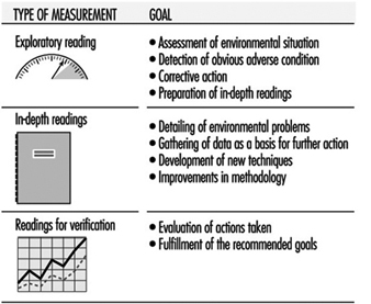
The traditional procedure in the field of workplace environmental control can be used to improve the quality of indoor air. It consists of identifying and quantifying a problem, proposing corrective measures, making sure that these measures are implemented, and then assessing their effectiveness after a period of time. This common procedure is not always the most adequate because often such an exhaustive evaluation, including the taking of many samples, is not necessary. Exploratory measures, which can range from a visual inspection to assaying of ambient air by direct reading methods, and which can provide an approximate concentration of pollutants, are sufficient for solving many of the existing problems. Once corrective measures have been taken, the results can be evaluated with a second measurement, and only when there is no clear evidence of an improvement a more thorough inspection (with in-depth measurements) or a complete analytical study can be undertaken (Swedish Work Environment Fund 1988).
The main advantages of such an exploratory procedure over the more traditional one are economy, speed and effectiveness. It requires competent and experienced personnel and the use of suitable equipment. Figure 1 summarizes the goals of the different stages of this procedure.
Figure 1. Planning the readings for exploratory evaluation.
Sampling Strategy
Analytical control of the quality of indoor air should be considered as a last resort only after the exploratory measurement has not given positive results, or if further evaluation or control of the initial tests is needed.
Assuming some previous knowledge of the sources of pollution and of the types of contaminants, the samples, even when limited in number, should be representative of the various spaces studied. Sampling should be planned to answer the questions What? How? Where? and When?
What
The pollutants in question must be identified in advance and, keeping in mind the different types of information that can be obtained, one should decide whether to make emission or immission measurements.
Emission measurements for indoor air quality can determine the influence of different sources of pollution, of climatic conditions, of the building’s characteristics, and of human intervention, which allow us to control or reduce the sources of emissions and improve the quality of indoor air. There are different techniques for taking this type of measurement: placing a collection system adjacent to the source of the emission, defining a limited work area and studying emissions as if they represented general working conditions, or working in simulated conditions applying monitoring systems that rely on head space measures.
Immission measurements allow us to determine the level of indoor air pollution in the different compartmentalized areas of the building, making it possible to produce a map of pollution for the entire structure. Using these measurements and identifying the different areas where people have carried out their activities and calculating the time they have spent at each task, it will be possible to determine the levels of exposure. Another way of doing this is by having individual workers wear monitoring devices while working.
It may be more practical, if the number of pollutants is large and varied, to select a few representative substances so that the reading is representative and not too expensive.
How
Selecting the type of reading to be made will depend on the available method (direct reading or sample-taking and analysis) and on the measuring technique: emission or immission.
Where
The location selected should be the most appropriate and representative for obtaining samples. This requires knowledge of the building being studied: its orientation relative to the sun, the number of hours it receives direct sunlight, the number of floors, the type of compartmentalization, if ventilation is natural or forced air, if its windows can be opened, and so on. Knowing the source of the complaints and the problems is also necessary, for example, whether they occur in the upper or the lower floors, or in the areas close to or far from the windows, or in the areas that have poor ventilation or illumination, among other locations. Selecting the best sites to draw the samples will be based on all of the available information regarding the above-mentioned criteria.
When
Deciding when to take the readings will depend on how concentrations of air pollutants change relative to time. Pollution may be detected first thing in the morning, during the workday or at the end of the day; it may be detected at the beginning or the end of the week; during the winter or the summer; when air-conditioning is on or off; as well as at other times.
To address these questions properly, the dynamics of the given indoor environment must be known. It is also necessary to know the goals of the measurements taken, which will be based on the types of pollutant that are being investigated. The dynamics of indoor environments are influenced by the diversity of the sources of pollution, the physical differences in the spaces involved, the type of compartmentalization, the type of ventilation and climate control used, outside atmospheric conditions (wind, temperature, season, etc.), and the building’s characteristics (number of windows, their orientation, etc.).
The goals of the measurements will determine if sampling will be carried out for short or long intervals. If the health effects of the given contaminants are thought to be long-term, it follows that average concentrations should be measured over long periods of time. For substances that have acute but not cumulative effects, measurements over short periods are sufficient. If intense emissions of short duration are suspected, frequent sampling over short periods is called for in order to detect the time of the emission. Not to be overlooked, however, is the fact that in many cases the possible choices in the type of sampling methods used may be determined by the analytical methods available or required.
If after considering all these questions it is not sufficiently clear what the source of the problem is, or when the problem occurs with greatest frequency, the decision as to where and when to take samples must be made at random, calculating the number of samples as a function of the expected reliability and cost.
Measuring techniques
The methods available for taking samples of indoor air and for their analysis can be grouped into two types: methods that involve a direct reading and those that involve taking samples for later analysis.
Methods based on a direct reading are those by which taking the sample and measuring the concentration of pollutants is done simultaneously; they are fast and the measurement is instantaneous, allowing for precise data at a relatively low cost. This group includes colorimetric tubes and specific monitors.
The use of colorimetric tubes is based on the change in the colour of a specific reactant when it comes in contact with a given pollutant. The most commonly used are tubes that contain a solid reactant and air is drawn through them using a manual pump. Assessing the quality of indoor air with colorimetric tubes is useful only for exploratory measurements and for measuring sporadic emissions since their sensitivity is generally low, except for some pollutants such as CO and CO2 that can be found at high concentrations in indoor air. It is important to keep in mind that the precision of this method is low and interference from unlooked-for contaminants is often a factor.
In the case of specific monitors, detection of pollutants is based on physical, electric, thermal, electromagnetic and chemoelectromagnetic principles. Most monitors of this type can be used to make measurements of short or long duration and gain a profile of contamination at a given site. Their precision is determined by their respective manufacturers and proper use demands periodic calibrations by means of controlled atmospheres or certified gas mixtures. Monitors are becoming increasingly precise and their sensitivity more refined. Many have built-in memory to store the readings, which can then be downloaded to computers for the creation of databases and the easy organization and retrieval of the results.
Sampling methods and analyses can be classified into active (or dynamic) and passive, depending on the technique.
With active systems, this pollution can be collected by forcing air through collecting devices in which the pollutant is captured, concentrating the sample. This is accomplished with filters, adsorbent solids, and absorbent or reactive solutions which are placed in bubblers or are impregnated onto porous material. Air is then forced through and the contaminant, or the products of its reaction, are analysed. For the analysis of air sampled with active systems the requirements are a fixative, a pump to move the air and a system to measure the volume of sampled air, either directly or by using flow and duration data.
The flow and the volume of sampled air are specified in the reference manuals or should be determined by previous tests and will depend on the quantity and type of absorbent or adsorbent used, the pollutants that are being measured, the type of measurement (emission or immission) and the condition of the ambient air during the taking of the sample (humidity, temperature, pressure). The efficacy of the collection increases by reducing the rate of intake or by increasing the amount of fixative used, directly or in tandem.
Another type of active sampling is the direct capture of air in a bag or any other inert and impermeable container. This type of sample gathering is used for some gases (CO, CO2, H2S, O2) and is useful as an exploratory measure when the type of pollutant is unknown. The drawback is that without concentrating the sample there may be insufficient sensitivity and further laboratory processing may be necessary to increase the concentration.
Passive systems capture pollutants by diffusion or permeation onto a base that may be a solid adsorbent, either alone or impregnated with a specific reactant. These systems are more convenient and easy to use than active systems. They do not require pumps to capture the sample nor highly trained personnel. But capturing the sample may take a long time and the results tend to furnish only medium concentration levels. This method cannot be used to measure peak concentrations; in those instances active systems should be used instead. To use passive systems correctly it is important to know the speed at which each pollutant is captured, which will depend on the diffusion coefficient of the gas or vapor and the design of the monitor.
Table 1 shows the salient characteristics of each sampling method and table 2 outlines the various methods used to gather and analyse the samples for the most significant indoor air pollutants.
Table 1. Methodology for taking samples
|
Characteristics |
Active |
Passive |
Direct reading |
|
Timed interval measurements |
+ |
+ |
|
|
Long-term measurements |
+ |
+ |
|
|
Monitoring |
+ |
||
|
Concentration of sample |
+ |
+ |
|
|
Immission measurement |
+ |
+ |
+ |
|
Emission measurement |
+ |
+ |
+ |
|
Immediate response |
+ |
+ Means that the given method is suitable to the method of measurement or desired measurement criteria.
Table 2. Detection methods for gases in indoor air
|
Pollutant |
Direct reading |
Methods |
Analysis |
||
|
Capture by diffusion |
Capture by concentration |
Direct capture |
|||
|
Carbon monoxide |
Electrochemical cell |
Bag or inert container |
GCa |
||
|
Ozone |
Chemiluminescence |
Bubbler |
UV-Visb |
||
|
Sulphur dioxide |
Electrochemical cell |
Bubbler |
UV-Vis |
||
|
Nitrogen dioxide |
Chemiluminescence |
Filter impregnated with a |
Bubbler |
UV-Vis |
|
|
Carbon dioxide |
Infrared spectroscopy |
Bag or inert container |
GC |
||
|
Formaldehyde |
— |
Filter impregnated with a |
Bubbler |
HPLCc |
|
|
VOCs |
Portable GC |
Adsorbent solids |
Adsorbent solids |
Bag or inert container |
GC (ECDd-FIDe-NPDf-PIDg) |
|
Pesticides |
— |
Adsorbent solids |
GC (ECD-FPD-NPD) |
||
|
Particulate matter |
— |
Optical sensor |
Filter |
Impactor |
Gravimetry |
— = Method unsuitable for pollutant.
a GC = gas chromatography.
b UV-Vis = visible ultraviolet spectrophotometry.
c HPLC = high precision liquid chromatography.
d CD = electron capture detector.
e FID = flame, ionization detector.
f NPD = nitrogen/phosphorous detector.
g PID = photoionization detector.
h MS = mass spectrometry.
Selecting the method
To select the best sampling method, one should first determine that validated methods for the pollutants being studied exist and see to it that the proper instruments and materials are available to gather and analyse the pollutant. One usually needs to know what their cost will be, and the sensitivity required for the job, as well as things that can interfere with the measurement, given the method chosen.
An estimate of the minimum concentrations of what one hopes to measure is very useful when evaluating the method used to analyse the sample. The minimum concentration required is directly related to the amount of pollutant that can be gathered given the conditions specified by the method used (i.e., the type of system used to capture the pollutant or the duration of sample taking and volume of air sampled). This minimum amount is what determines the sensitivity required of the method used for analysis; it can be calculated from reference data found in the literature for a particular pollutant or group of pollutants, if they were arrived at by a similar method to the one that will be used. For example, if it is found that hydrocarbon concentrations of 30 (mg/m3) are commonly found in the area under study, the analytical method used should allow the measurement of those concentrations easily. If the sample is obtained with a tube of active carbon in four hours and with a flow of 0.5 litres per minute, the amount of hydrocarbons gathered in the sample is calculated by multiplying the flow rate of the substance by the period of time monitored. In the given example this equals:
![]() of hydrocarbons
of hydrocarbons ![]()
Any method for detecting hydrocarbons that requires the amount in the sample to be under 3.6 μg can be used for this application.
Another estimate could be calculated from the maximum limit established as the allowable limit for indoor air for the pollutant being measured. If these figures don’t exist and the usual concentrations found in indoor air are not known, nor the rate at which the pollutant is being discharged into the space, approximations can be used based on the potential levels of the pollutant that can negatively affect health. The method chosen should be capable of measuring 10% of the established limit or of the minimal concentration that could affect health. Even if the method of analysis chosen has an acceptable degree of sensitivity, it is possible to find concentrations of pollutants that are below the lower limit of detection of the chosen method. This should be kept in mind when calculating average concentrations. For example, if out of ten readings taken three are below the detection limit, two averages should be calculated, one assigning these three readings the value of zero and another giving them the lowest detection limit, which renders a minimum average and a maximum average. The true measured average will be found between the two.
Analytical Procedures
The number of indoor air pollutants is great and they are found in small concentrations. The methodology that has been available is based on adapting methods used to monitor the quality of outdoor, atmospheric, air and air found in industrial situations. Adapting these methods for the analysis of indoor air implies changing the range of the concentration sought, when the method allows, using longer sampling times and greater amounts of absorbents or adsorbents. All these changes are appropriate when they do not lead to a loss in reliability or precision. Measuring a mixture of contaminants is usually expensive and the results obtained imprecise. In many cases all that will be ascertained will be a pollution profile that will indicate the level of contamination during sampling intervals, compared to clean air, to outside air, or to other indoor spaces. Direct reading monitors are used to monitor the pollution profile and may not be suitable if they are too noisy or too large. Ever smaller and quieter monitors, that afford greater precision and sensitivity, are being designed. Table 3 shows in outline the current state of the methods used to measure the different types of contaminants.
Table 3. Methods used for the analysis of chemical pollutants
|
Pollutant |
Direct-reading monitora |
Sampling and analysis |
|
Carbon monoxide |
+ |
+ |
|
Carbon dioxide |
+ |
+ |
|
Nitrogen dioxide |
+ |
+ |
|
Formaldehyde |
– |
+ |
|
Sulphur dioxide |
+ |
+ |
|
Ozone |
+ |
+ |
|
VOCs |
+ |
+ |
|
Pesticides |
– |
+ |
|
Particulates |
+ |
+ |
a ++ = most commonly used; + = less commonly used; – = not applicable.
Analysis of gases
Active methods are the most common for the analysis of gases, and are carried out using absorbent solutions or adsorbent solids, or by directly taking a sample of air with a bag or some other inert and airtight container. In order to prevent loss of part of the sample and increase the accuracy of the reading, the volume of the sample must be lower and the amount of absorbent or adsorbent used should be more than for other types of pollution. Care should also be taken in transporting and storing the sample (keeping it at low temperature) and minimizing the time before the sample is tested. Direct reading methods are widely used for measuring gases because of the considerable improvement in the capabilities of modern monitors, which are more sensitive and more precise than before. Because of their ease of use and the level and type of information that they furnish, they are increasingly replacing traditional methods of analysis. Table 4 shows the minimum detection levels for the various gases studied given the method of sampling and analysis used.
Table 4. Lower detection limits for some gases by monitors used to assess indoor air quality
|
Pollutant |
Direct-reading monitora |
Sample-taking and |
|
Carbon monoxide |
1.0 ppm |
0.05 ppm |
|
Nitrogen dioxide |
2 ppb |
1.5 ppb (1 week)b |
|
Ozone |
4 ppb |
5.0 ppb |
|
Formaldehyde |
5.0 ppb (1 week)b |
a Carbon dioxide monitors that use infrared spectroscopy are always sensitive enough.
b Passive monitors (length of exposure).
These gases are common pollutants in indoor air. They are measured by using monitors that detect them directly by electrochemical or infrared means, even though infrared detectors are not very sensitive. They can also be measured by taking air samples directly with inert bags and analysing the sample by gas chromatography with a flame ionization detector, transforming the gases into methane first by means of a catalytic reaction. Thermal conduction detectors are usually sensitive enough to measure normal concentrations of CO2.
Nitrogen dioxide
Methods have been developed to detect nitrogen dioxide, NO2, in indoor air by using passive monitors and taking samples for later analysis, but these methods have presented sensitivity problems that will hopefully be overcome in the future. The best known method is the Palmes tube, which has a detection limit of 300 ppb. For non-industrial situations, sampling should be for a minimum of five days in order to obtain a detection limit of 1.5 ppb, which is three times the value of the blank for a one-week exposure. Portable monitors that measure in real time have also been developed based on the chemiluminescence reaction between NO2 and the reactant luminol, but the results obtained by this method can be affected by temperature and their linearity and sensitivity depend on the characteristics of the solution of luminol used. Monitors that have electrochemical sensors have improved sensitivity but are subject to interference from compounds that contain sulphur (Freixa 1993).
Sulphur dioxide
A spectrophotometric method is used to measure sulphur dioxide, SO2, in an indoor environment. The air sample is bubbled through a solution of potassium tetrachloromercuriate to form a stable complex which is in turn measured spectrophotometrically after reacting with pararosaniline. Other methods are based on flame photometry and pulsating ultraviolet fluorescence, and there are also methods based on deriving the measurement before the spectroscopic analysis. This type of detection, which has been used for outside air monitors, is not suited for indoor air analysis because of a lack of specificity and because many of these monitors require a venting system to eliminate the gases that they generate. Because emissions of SO2 have been greatly reduced and it is not considered an important pollutant of indoor air, the development of monitors for its detection have not advanced very much. However, there are portable instruments available on the market that can detect SO2 based on the detection of pararosaniline (Freixa 1993).
Ozone
Ozone, O3, can only be found in indoor environments in special situations in which it is generated continuously, since it decays rapidly. It is measured by direct reading methods, by colorimetric tubes and by chemiluminescence methods. It can also be detected by methods used in industrial hygiene that can be easily adapted for indoor air. The sample is obtained with an absorbent solution of potassium iodide in a neutral medium and then subjected to spectrophotometric analysis.
Formaldehyde
Formaldehyde is an important pollutant of indoor air, and because of its chemical and toxic characteristics an individualized evaluation is recommended. There are different methods for detecting formaldehyde in air, all of them based on taking samples for later analysis, with active fixing or by diffusion. The most appropriate capturing method will be determined by the type of sample (emission or immission) used and the sensitivity of the analytical method. The traditional methods are based on obtaining a sample by bubbling air through distilled water or a solution of 1% sodium bisulphate at 5°C, and then analysing it with spectrofluorometric methods. While the sample is stored, it should also be kept at 5°C. SO2 and the components of tobacco smoke can create interference. Active systems or methods that capture pollutants by diffusion with solid adsorbents are used more and more frequently in indoor air analysis; they all consist of a base that can be a filter or a solid saturated with a reactant, such as sodium bisulphate or 2,4-diphenylhydrazine. Methods that capture the pollutant by diffusion, in addition to general advantages of that method, are more sensitive than active methods because the time required to obtain the sample is longer (Freixa 1993).
Detection of volatile organic compounds (VOCs)
The methods used to measure or monitor organic vapors in indoor air must meet a series of criteria: they should have a sensitivity in the order of parts per billion (ppb) to parts per trillion (ppt), the instruments used to take the sample or make a direct reading must be portable and easy to handle in the field, and the results obtained must be precise and capable of being duplicated. There are a great many methods that meet these criteria, but the ones most frequently used to analyse indoor air are based on sample taking and analysis. Direct detection methods exist that consist of portable gas chromatographs with different detection methods. These instruments are expensive, their handling is sophisticated and they can be operated only by trained personnel. For polar and nonpolar organic compounds that have a boiling point between 0°C and 300°C, the most widely used adsorbent both for active and passive sampling systems has been activated carbon. Porous polymers and polymer resins, such as Tenax GC, XAD-2 and Ambersorb are also used. The most widely used of these is Tenax. The samples obtained with activated carbon are extracted with carbon disulphide and they are analysed by gas chromatography with flame ionization, electron-capture, or mass spectrometry detectors, followed by qualitative and quantitative analysis. Samples obtained with Tenax are usually extracted by thermal desorption with helium and are condensed in a nitrogen cold trap before being fed to the chromatograph. Another common method consists in obtaining samples directly, using bags or inert containers, feeding the air directly to the gas chromatograph, or concentrating the sample first with an adsorbent and a cold trap. The detection limits of these methods depend on the compound analysed, the volume of the sample taken, the background pollution and the detection limits of the instrument used. Because quantifying each and every one of the compounds present is impossible, quantification is normally done by families, by using as a reference compounds that are characteristic of each family of compounds. In detecting VOCs in indoor air, the purity of the solvents used is very important. If thermal desorption is used, the purity of the gases is also important.
Detection of pesticides
To detect pesticides in indoor air, the methods commonly employed consist of taking samples with solid adsorbents, although the use of bubblers and mixed systems is not ruled out. The solid adsorbent most commonly used has been porous polymer Chromosorb 102, although polyurethane foams (PUFs) that can capture a wider number of pesticides are being used more and more. The methods of analysis vary according to the sampling method and the pesticide. Usually they are analysed by using gas chromatography with different specific detectors, from electron capture to mass spectrometry. The potential of the latter for identifying compounds is considerable. The analysis of these compounds presents certain problems, which include the contamination of glass parts in the sample-taking systems with traces of polychlorinated biphenyls (PCBs), phthalates or pesticides.
Detection of environmental dust or particles
For the capture and analysis of particles and fibres in air a great variety of techniques and equipment are available and suited for assessing indoor air quality. Monitors that permit a direct reading of the concentration of particles in the air use diffuse light detectors, and methods that employ sample taking and analysis use weighting and analysis with a microscope. This type of analysis requires a separator, such as a cyclone or an impactor, to sift out larger particles before a filter can be used. Methods that employ a cyclone can handle small volumes, which results in long sessions of sample taking. Passive monitors offer excellent precision, but they are affected by ambient temperature and tend to give readings with higher values when the particles are small.
Smoking Regulations
In regard to taking action to reduce the use of tobacco, governments should keep in mind that while people decide on their own whether they should stop smoking, it is a government’s responsibility to take all the necessary measures to encourage them to stop. The steps taken by legislators and governments of many countries have been indecisive, because while the reduction in the use of tobacco is an undisputed improvement in public health—with attendant savings in public health expenditures—there would be a series of economic losses and dislocations in many sectors, at least of a temporary nature. The pressure that international health and environmental organizations and agencies can exert in this regard is very important, because many countries may water down measures against the use of tobacco because of economic problems—especially if tobacco is an important source of income.
This article briefly describes regulatory measures that can be adopted to reduce smoking in a country.
Warnings on Cigarette Packs
One of the first measures adopted in many countries is to require that cigarette packs prominently display the warning that smoking seriously injures the smoker’s health. This warning, whose aim is not so much to exert an immediate effect on the smoker, but rather to show that the government is concerned about the problem, is creating a psychological climate that will favour the adoption of later measures that otherwise would be considered aggressive by the smoking population.
Some experts advocate the inclusion of these warnings on cigars and pipe tobacco. But the more general opinion is that those warnings are unnecessary, because people who use that type of tobacco do not normally inhale the smoke, and extending these warnings would lead more likely to a disregard of the messages as a whole. This is why the prevalent opinion is that the warnings should be applied only to cigarette packs. A reference to second-hand smoke has not, for the moment, been considered, but it is not an option that should be discarded.
Smoking Restrictions in Public Spaces
Forbidding smoking in public spaces is one of the most effective regulatory instruments. These prohibitions can significantly reduce the number of people exposed to second-hand smoke and, in addition, can reduce smokers’ daily cigarette consumption. The common complaints by owners of public spaces, such as hotels, restaurants, recreational facilities, dance halls, theatres and so forth, are based on the argument that these measures will result in a loss of customers. However, if governments implement these measures across the board, the negative impact of a loss of clientele will occur only in the first phase, because people will eventually adapt to the new situation.
Another possibility is the design of specific spaces for smokers. The separation of smokers from non-smokers should be effective in order to obtain the desired benefits, creating barriers that prevent non-smokers from inhaling tobacco smoke. Separation must thus be physical and, if the air-conditioning system uses recycled air, the air from smoking areas should not be mixed with that from non-smoking areas. Creating spaces for smokers therefore implies construction and compartmentalization expenses, but may be a solution for those who want to serve the smoking public.
Aside from locations where smoking is obviously forbidden for security reasons because of possible explosion or fire, there should also be areas—such as health care and sports facilities, schools and day-care centres—where smoking is not permitted even though there are no safety risks of that kind.
Smoking Restrictions at Work
Smoking restrictions in the workplace may also be considered in light of the above. Governments and business owners, together with trade unions, can establish programmes to reduce the use of tobacco at work. Campaigns to curtail smoking at work are generally successful.
Whenever possible, creating non-smoking areas to establish a policy against tobacco use and to support people who defend the right not to be second-hand smokers is recommended. In case of a conflict between a smoker and a non-smoker, regulations should always allow the non-smoker to prevail, and whenever they cannot be separated, the smoker should be pressured to abstain from smoking at the workstation.
In addition to places where for health or safety reasons smoking should be forbidden, the possibility of synergism between the effects of chemical pollution in the workplace and tobacco smoke should not be ignored in other areas either. The weight of such considerations will result, without a doubt, in a broad extension of smoking restrictions, especially in industrial workplaces.
Greater Economic Pressure against Tobacco
Another regulatory tool governments rely on to curb the use of tobacco is levying higher taxes, chiefly on cigarettes. This policy is intended to lead to lower tobacco consumption, which would justify the inverse relation between the price of tobacco and its consumption and which can be measured when comparing the situation in different countries. It is considered effective where the population is forewarned of the dangers of tobacco use and advised of the need to stop consuming it. An increase in the price of tobacco can be a motivation to quit smoking. This policy, however, has many opponents, who base their criticisms on arguments briefly mentioned below.
In the first place, according to many specialists, the increase in the price of tobacco for fiscal reasons is followed by a temporary reduction in the use of tobacco, followed by a gradual return to the previous consumption levels as the smokers get used to the new price. In other words, smokers assimilate a rise in the price of tobacco much in the same way that people get used to other taxes or to the rise in the cost of living.
In the second place, a shift in the habits of smokers has also been observed. When prices go up they tend to seek out cheaper brands of lower quality that probably also pose a greater risk to their health (because they lack filters or have higher amounts of tar and nicotine). This shift may go so far as to induce smokers to adopt the practice of making home-made cigarettes, which would completely eliminate any possibility of controlling the problem.
In the third place, many experts are of the opinion that measures of this kind tend to bolster the belief that the government accepts tobacco and its consumption as yet another means to collect taxes, leading to the contradictory belief that what the government really wants is that people smoke so that it can collect more money with the special tax on tobacco.
Limiting Publicity
Another weapon used by governments to reduce tobacco consumption is to restrict or simply forbid any publicity for the product. Governments and many international organizations have a policy of forbidding publicity for tobacco in certain spheres, such as sports (at least some sports), health care, the environment, and education. This policy has unquestionable benefits, which are especially effective when it eliminates publicity in those environments that affect young people at a time when they are likely to take up the smoking habit.
Public Programmes that Encourage People to QuitSmoking
The use of anti-smoking campaigns as a normal practice, adequately funded and organized as a rule of conduct in certain spheres, such as the world of work, has been shown to be highly successful.
Campaigns to Educate Smokers
Complementing what was said above, educating smokers so that they will smoke “better” and cut down on their consumption of cigarettes is another avenue available to governments to reduce the adverse health effects of tobacco use on the population. These efforts should be directed at reducing the daily consumption of cigarettes, at inhibiting the inhalation of smoke as much as possible, at not smoking the butts of cigarettes (the toxicity of smoke increases towards the end of the cigarette), at not keeping the cigarette steadily at the lips, and at adopting preferences for brands with lower tar and nicotine.
Measures of this type evidently do not reduce the number of smokers, but they do reduce how much smokers are harmed by their habit. There are arguments against this type of remedy because it may give the impression that smoking is not intrinsically a bad habit, since smokers are told how best to smoke.
Concluding Remarks
Regulatory and legislative action by different governments is slow and not sufficiently effective, especially given what would be required due to the problems caused by tobacco use. Often this is the case because of legal hurdles against implementing such measures, arguments against unfair competition, or even the protection of the individual’s right to smoke. Progress in the use of regulations has been slow but it is nonetheless steady. On the other hand, the difference between active smokers and second-hand or passive smokers should be kept in mind. All the measures that would help someone to stop smoking, or at least to reduce daily consumption effectively, should be directed at the smoker; all the weight of regulations should be brought to bear against this habit. The passive smoker should be given every possible argument to support his or her right not to inhale tobacco smoke, and to defend the right to enjoy the use of smoke-free environments at home, at work and at play.
Tobacco Smoke
In 1985 the Surgeon General of the US Public Health Service reviewed the health consequences of smoking with regard to cancer and chronic lung disease in the workplace. It was concluded that for most US workers, cigarette smoking represents a greater cause of death and disability than their workplace environment. However, the control of smoking and a reduction of the exposure to hazardous agents at the workplace are essential, since these factors often act synergistically with smoking in the induction and development of respiratory diseases. Several occupational exposures are known to induce chronic bronchitis in workers. These include exposures to dust from coal, cement and grain, to silica aerosols, to vapors generated during welding, and to sulphur dioxide. Chronic bronchitis among workers in these occupations is often aggravated by cigarette smoking (US Surgeon General 1985).
Epidemiological data have clearly documented that uranium miners and asbestos workers who smoke cigarettes carry significantly higher risks of cancer of the respiratory tract than non-smokers in these occupations. The carcinogenic effect of uranium and asbestos and cigarette smoking is not merely additive, but synergistic in inducing squamous cell carcinoma of the lung (US Surgeon General 1985; Hoffmann and Wynder 1976; Saccomanno, Huth and Auerbach 1988; Hilt et al. 1985). The carcinogenic effects of exposure to nickel, arsenicals, chromate, chloromethyl ethers, and those of cigarette smoking are at least additive (US Surgeon General 1985; Hoffmann and Wynder 1976; IARC 1987a, Pershagen et al. 1981). One would assume that coke-oven workers who smoke have a higher risk of lung and kidney cancer than non-smoking coke-oven workers; however, we lack epidemiological data that substantiate this concept (IARC 1987c).
It is the aim of this overview to evaluate the toxic effects of the exposure of men and women to environmental tobacco smoke (ETS) at the workplace. Certainly, curtailing smoking at the workplace will benefit active smokers by reducing their consumption of cigarettes during the workday, thereby increasing the possibility that they become ex-smokers; but smoking cessation will also be of benefit to those non-smokers who are allergic to tobacco smoke or who have pre-existing lung or heart ailments.
Physico-Chemical Nature of EnvironmentalTobacco Smoke
Mainstream and sidestream smoke
ETS is defined as the material in indoor air that originates from tobacco smoke. Although pipe and cigar smoking contribute to ETS, cigarette smoke is generally the major source. ETS is a composite aerosol that is emitted primarily from the burning cone of a tobacco product between puffs. This emission is called sidestream smoke (SS). To a minor extent, ETS consists also of mainstream smoke (MS) constituents, that is, those that are exhaled by the smoker. Table 7 lists the ratios of major toxic and carcinogenic agents in the smoke that is inhaled, the mainstream smoke, and in the sidestream smoke (Hoffmann and Hecht 1990; Brunnemann and Hoffmann 1991; Guerin et al. 1992; Luceri et al. 1993). Under “Type of toxicity”, smoke components marked “C” represent animal carcinogens that are recognized by the International Agency for Research on Cancer (IARC). Among these are benzene,β-naphthylamine, 4-aminobiphenyl and polonium-210, which are also established human carcinogens (IARC 1987a; IARC 1988). When filter cigarettes are being smoked, certain volatile and semi-volatile components are selectively removed from the MS by filter tips (Hoffmann and Hecht 1990). However, these compounds occur in far higher amounts in undiluted SS than in MS. Furthermore, those smoke components that are favoured to be formed during smouldering in the reducing atmosphere of the burning cone, are released into SS to a far greater extent than into MS. This includes groups of carcinogens like the volatile nitrosamines, tobacco-specific nitrosamines (TSNA) and aromatic amines.
Table 1. Some toxic and tumorigenic agents in undiluted cigarette sidestream smoke
|
Compound |
Type of |
Amount in |
Ratio of side- |
|
Vapour phase |
|||
|
Carbon monoxide |
T |
26.80-61 mg |
2.5-14.9 |
|
Carbonyl sulphide |
T |
2-3 μg |
0.03-0.13 |
|
1,3-Butadiene |
C |
200-250 μg |
3.8-10.8 |
|
Benzene |
C |
240-490 μg |
8-10 |
|
Formaldehyde |
C |
300-1,500 μg |
10-50 |
|
Acrolein |
T |
40-100 μg |
8-22 |
|
3-Vinylpyridine |
T |
330-450 μg |
24-34 |
|
Hydrogen cyanide |
T |
14-110 μg |
0.06-0.4 |
|
Hydrazine |
C |
90 ng |
3 |
|
Nitrogen oxides (NOx) |
T |
500-2,000 μg |
3.7-12.8 |
|
N-Nitrosodimethylamine |
C |
200-1,040 ng |
12-440 |
|
N-Nitrosodiethylamine |
C |
NDb-1,000 ng |
<40 |
|
N-Nitrosopyrrolidine |
C |
7-700 ng |
4-120 |
|
Particulate phase |
|||
|
Tar |
C |
14-30 mg |
1.1-15.7 |
|
Nicotine |
T |
2.1-46 mg |
1.3-21 |
|
Phenol |
TP |
70-250 μg |
1.3-3.0 |
|
Catechol |
CoC |
58-290 μg |
0.67-12.8 |
|
2-Toluidine |
C |
2.0-3.9 μg |
18-70 |
|
β-Naphthylamine |
C |
19-70 ng |
8.0-39 |
|
4-Aminobiphenyl |
C |
3.5-6.9 ng |
7.0-30 |
|
Benz(a)anthracene |
C |
40-200 ng |
2-4 |
|
Benzo(a)pyrene |
C |
40-70 ng |
2.5-20 |
|
Quinoline |
C |
15-20 μg |
8-11 |
|
NNNc |
C |
0.15-1.7 μg |
0.5-5.0 |
|
NNKd |
C |
0.2-1.4 μg |
1.0-22 |
|
N-Nitrosodiethanolamine |
C |
43 ng |
1.2 |
|
Cadmium |
C |
0.72 μg |
7.2 |
|
Nickel |
C |
0.2-2.5 μg |
13-30 |
|
Zinc |
T |
6.0 ng |
6.7 |
|
Polonium-210 |
C |
0.5-1.6 pCi |
1.06-3.7 |
a C=Carcinogenic; CoC=co-carcinogenic; T=toxic; TP=tumor promoter.
b ND=not detected.
c NNN=N‘-nitrosonornicotine.
d NNK=4-(methylnitrosamino)-1-(3-pyridyl)-1-butanone.
ETS in indoor air
Although undiluted SS contains higher amounts of toxic and carcinogenic components than MS, the SS inhaled by non-smokers is highly diluted by air and its properties are altered because of the decay of certain reactive species. Table 8 lists reported data for toxic and carcinogenic agents in indoor air samples of various degrees of tobacco smoke pollution (Hoffmann and Hecht 1990; Brunnemann and Hoffmann 1991; Luceri et al. 1993). The air dilution of SS has a significant impact on the physical characteristics of this aerosol. In general, the distribution of various agents between vapor phase and particulate phase is changed in favour of the former. The particles in ETS are smaller (<0.2 μ) than those in MS (~0.3 μ) and the pH levels of SS (pH 6.8 - 8.0) and of ETS are higher than the pH of MS (5.8 - 6.2; Brunnemann and Hoffmann 1974). Consequently, 90 to 95% of nicotine is present in the vapor phase of ETS (Eudy et al. 1986). Similarly, other basic components such as the minor Nicotiana alkaloids, as well as amines and ammonia, are present mostly in the vapor phase of ETS (Hoffmann and Hecht 1990; Guerin et al. 1992).
Table 2. Some toxic and tumorigenic agents in indoor environments polluted by tobacco smoke
|
Pollutant |
Location |
Concentration/m3 |
|
Nitric oxide |
Workrooms |
50-440 μg |
|
Nitrogen dioxide |
Workrooms |
68-410 μg |
|
Hydrogen cyanide |
Living-rooms |
8-122 μg |
|
1,3-Butadiene |
Bars |
2.7-4.5 μg |
|
Benzene |
Public places |
20-317 μg |
|
Formaldehyde |
Living-rooms |
2.3-5.0 μg |
|
Acrolein |
Public places |
30-120 μg |
|
Acetone |
Coffee houses |
910-1,400 μg |
|
Phenols (volatile) |
Coffee houses |
7.4-11.5 ng |
|
N-Nitrosodimethylamine |
Bars, restaurants, offices |
<10-240 ng |
|
N-Nitrosodiethylamine |
Restaurants |
<10-30 ng |
|
Nicotine |
Residences |
0.5-21 μg |
|
2-Toluidine |
Offices |
3.0-12.8 ng |
|
b-Naphthylamine |
Offices |
0.27-0.34 ng |
|
4-Aminobiphenyl |
Offices |
0.1 ng |
|
Benz(a)anthracene |
Restaurants |
1.8-9.3 ng |
|
Benzo(a)pyrene |
Restaurants |
2.8-760 μg |
|
NNNa |
Bars |
4.3-22.8 ng |
|
NNKc |
Bars |
9.6-23.8 ng |
a NNN=N‘-nitrosonornicotine.
b ND=not detected.
c NNK=4-(methylnitrosamino)-1-(3-pyridyl)-1-butanone.
Biomarkers of the Uptake of ETS by Non-Smokers
Although a significant number of non-smoking workers are exposed to ETS at the workplace, in restaurants, in their own homes or in other indoor places, it is hardly possible to estimate the actual uptake of ETS by an individual. ETS exposure can be more precisely determined by measuring specific smoke constituents or their metabolites in physiological fluids or in exhaled air. Although several parameters have been explored, such as CO in exhaled air, carboxyhaemoglobin in blood, thiocyanate (a metabolite of hydrogen cyanide) in saliva or urine, or hydroxyproline and N-nitrosoproline in urine, only three measures are actually helpful for estimating the uptake of ETS by non-smokers. They allow us to distinguish passive smoke exposure from that of active smokers and from non-smokers who have absolutely no exposure to tobacco smoke.
The most widely used biomarker for ETS exposure of non-smokers is cotinine, a major nicotine metabolite. It is determined by gas chromatography, or by radioimmunoassay in blood or preferably urine, and reflects the absorption of nicotine through the lung and oral cavity. A few millilitres of urine from passive smokers is sufficient to determine cotinine by either of the two methods. In general, a passive smoker has cotinine levels of 5 to 10 ng/ml of urine; however, higher values have occasionally been measured for non-smokers who were exposed to heavy ETS over a longer period. A dose response has been established between duration of ETS exposure and urinary cotinine excretion (table 3, Wald et al. 1984). In most field studies, cotinine in the urine of passive smokers amounted to between 0.1 and 0.3% of the mean concentrations found in the urine of smokers; however, upon prolonged exposure to high concentrations of ETS, cotinine levels have corresponded to as much as 1% of the levels measured in the urine of active smokers (US National Research Council 1986; IARC 1987b; US Environmental Protection Agency 1992).
Table 3. Urinary cotinine in non-smokers according to the number of reported hours of exposure to other people’s tobacco smoke within the previous seven days
|
Duration of exposure |
|||
|
Quintile |
Limits (hrs) |
Number |
Urinary cotinine (mean ± SD) |
|
1st |
0.0-1.5 |
43 |
2.8±3.0 |
|
2nd |
1.5-4.5 |
47 |
3.4±2.7 |
|
3rd |
4.5-8.6 |
43 |
5.3±4.3 |
|
4th |
8.6-20.0 |
43 |
14.7±19.5 |
|
5th |
20.0-80.0 |
45 |
29.6±73.7 |
|
All |
0.0-80.0 |
221 |
11.2±35.6 |
a Trend with increasing exposure was significant (p<0.001).
Source: Based on Wald et al. 1984.
The human bladder carcinogen 4-aminobiphenyl, which transfers from tobacco smoke into ETS, has been detected as a haemoglobin adduct in passive smokers in concentrations up to 10% of the mean adduct level found in smokers (Hammond et al. 1993). Up to 1% of the mean levels of a metabolite of the nicotine-derived carcinogen 4-(methylnitrosamino)-1-(3-pyridyl)-1-butanone (NNK), which occurs in the urine of cigarette smokers, has been measured in the urine of non-smokers who had been exposed to high concentrations of SS in a test laboratory (Hecht et al. 1993). Although the latter biomarker method has not as yet been applied in field studies, it holds promise as a suitable indicator of the exposure of non-smokers to a tobacco-specific lung carcinogen.
Environmental Tobacco Smoke and Human Health
Disorders other than cancer
Prenatal exposure to MS and/or ETS and early postnatal exposure to ETS increase the probability of complications during viral respiratory infections in children during the first year of life.
The scientific literature contains several dozens of clinical reports from various countries, reporting that children of parents who smoke, especially children under the age of two years, show an excess of acute respiratory illness (US Environmental Protection Agency 1992; US Surgeon General 1986; Medina et al. 1988; Riedel et al. 1989). Several studies also described an increase of middle ear infections in children who had exposure to parental cigarette smoke. The increased prevalence of middle ear effusion attributable to ETS led to increased hospitalization of young children for surgical intervention (US Environmental Protection Agency 1992; US Surgeon General 1986).
In recent years, sufficient clinical evidence has led to the conclusion that passive smoking is associated with increased severity of asthma in those children who already have the disease, and that it most likely leads to new cases of asthma in children (US Environmental Protection Agency 1992).
In 1992, the US Environmental Protection Agency (1992) critically reviewed the studies on respiratory symptoms and lung functions in adult non-smokers exposed to ETS, concluding that passive smoking has subtle but statistically significant effects on the respiratory health of non-smoking adults.
A search of the literature on the effect of passive smoking on respiratory or coronary diseases in workers revealed only a few studies. Men and women who were exposed to ETS at the workplace (offices, banks, academic institutions, etc.) for ten or more years had impaired pulmonary function (White and Froeb 1980; Masi et al. 1988).
Lung cancer
In 1985, the International Agency for Research on Cancer (IARC) reviewed the association of passive tobacco smoke exposure with lung cancer in non-smokers. Although in some studies, each non-smoker with lung cancer who had reported ETS exposure was personally interviewed and had supplied detailed information on exposure (US National Research Council 1986; US EPA 1992; US Surgeon General 1986; Kabat and Wynder 1984), the IARC concluded:
The observations on non-smokers that have been made so far, are compatible with either an increased risk from ‘passive’ smoking, or an absence of risk. Knowledge of the nature of sidestream and mainstream smoke, of the materials absorbed during ‘passive’ smoking and of the quantitative relationship between dose and effect that are commonly observed from exposure to carcinogens, however, leads to the conclusion that passive smoking gives rise to some risk of cancer (IARC 1986).
Thus, there is an apparent dichotomy between experimental data which support the concept that ETS gives rise to some risk of cancer, and epidemiological data, which are not conclusive with respect to ETS exposure and cancer. Experimental data, including biomarker studies, have further strengthened the concept that ETS is carcinogenic, as was discussed earlier. We will now discuss how far the epidemiological studies that have been completed since the cited IARC report have contributed to a clarification of the ETS lung cancer issue.
According to the earlier epidemiological studies, and in about 30 studies reported after 1985, ETS exposure of non-smokers constituted a risk factor for lung cancer of less than 2.0, relative to the risk of a non-smoker without significant ETS exposure (US Environmental Protection Agency 1992; Kabat and Wynder 1984; IARC 1986; Brownson et al. 1992; Brownson et al. 1993). Few, if any, of these epidemiological studies meet the criteria of causality in the association between an environmental or occupational factor and lung cancer. Criteria that fulfil these requirements are:
- a well-established degree of association (risk factor≥3)
- reproducibility of the observation by a number of studies
- agreement between duration of exposure and effect
- biological plausibility.
One of the major uncertainties about the epidemiological data lies in the limited reliability of the answers obtained by questioning cases and/or their next-of-kin with regard to the smoking habits of the cases. It appears that there is generally an accord between parental and spousal smoking histories provided by cases and controls; however, there are low agreement rates for duration and intensity of smoking (Brownson et al. 1993; McLaughlin et al. 1987; McLaughlin et al. 1990). Some investigators have challenged the reliability of the information derived from individuals about their smoking status. This is exemplified by a large-scale investigation carried out in southern Germany. A randomly selected study population consisted of more than 3,000 men and women, ranging in age from 25 to 64 years. These same people were questioned three times in 1984-1985, in 1987-1988 and again in 1989-1990 as to their smoking habits, while each time urine was collected from each proband and was analysed for cotinine. Those volunteers who were found to have more than 20 ng of cotinine per ml of urine were considered to be smokers. Among 800 ex-smokers who claimed to be non-smokers, 6.3%, 6.5% and 5.2% had cotinine levels above 20 ng/ml during the three time periods tested. The self-proclaimed never-smokers, who were identified as actual smokers according to cotinine analyses, constituted 0.5%, 1.0% and 0.9%, respectively (Heller et al. 1993).
The limited reliability of the data obtained by questionnaire, and the relatively limited number of non-smokers with lung cancer who were not exposed to carcinogens at their workplaces, point to the need for a prospective epidemiological study with assessment of biomarkers (e.g., cotinine, metabolites of polynuclear aromatic hydrocarbons, and/or metabolites of NNK in urine) to bring about a conclusive evaluation of the question on causality between involuntary smoking and lung cancer. While such prospective studies with biomarkers represent a major task, they are essential in order to answer the questions on exposure which have major public health implications.
Environmental Tobacco Smoke and the Occupational Environment
Although epidemiological studies have thus far not demonstrated a causal association between ETS exposure and lung cancer, it is nevertheless highly desirable to protect workers at the site of employment from exposure to environmental tobacco smoke. This concept is supported by the observation that long-term exposure of non-smokers to ETS at the workplace can lead to reduced pulmonary function. Furthermore, in occupational environments with exposure to carcinogens, involuntary smoking may increase the risk of cancer. In the United States, the Environmental Protection Agency has classified ETS as a Group A (known human) carcinogen; therefore, the law in the United States requires that employees be protected against exposure to ETS.
Several measures can be taken to protect the non-smoker from exposure to ETS: prohibiting smoking at the worksite, or at least separating smokers from non-smokers where possible, and assuring that the smokers’ rooms have a separate exhaust system. The most rewarding and by far the most promising approach is to assist employees who are cigarette smokers in cessation efforts.
The worksite can offer excellent opportunities for implementing smoking cessation programmes; in fact, numerous studies have shown that worksite programmes are more successful than clinic-based programmes, because employer-sponsored programmes are more intense in nature and they offer economic and/or other incentives (US Surgeon General 1985). It is also indicated that the elimination of occupationally related chronic lung diseases and cancer frequently cannot proceed without efforts to convert the workers into ex-smokers. Furthermore, worksite interventions, including smoking cessation programmes, can produce lasting changes in reducing some cardiovascular risk factors for the employees (Gomel et al. 1993).
We greatly appreciate the editorial assistance of Ilse Hoffmann and the preparation of this manuscript by Jennifer Johnting. These studies are supported by USPHS Grants CA-29580 and CA-32617 from the National Cancer Institute.
Radon
Most of the radiation that a human being will be exposed to during a lifetime comes from natural sources in outer space or from materials present in the earth’s crust. Radioactive materials may affect the organism from without or, if inhaled or ingested with food, from within. The dose received may be very variable because it depends, on the one hand, on the amount of radioactive minerals present in the area of the world where the person lives—which is related to the amount of radioactive nuclides in the air and the amount found both in food and especially in drinking water—and, on the other, on the use of certain construction materials and the use of gas or coal for fuel, as well as the type of construction employed and the traditional habits of people in the given locality.
Today, radon is considered the most prevalent source of natural radiation. Together with its “daughters," or radionuclides formed by its disintegration, radon constitutes approximately three fourths of the effective equivalent dose to which humans are exposed due to natural terrestrial sources. The presence of radon is associated with an increase in the occurrence of lung cancer due to the deposition of radioactive substances in the bronchial region.
Radon is a colourless, odourless and tasteless gas seven times as heavy as air. Two isotopes occur most frequently. One is radon-222, a radionuclide present in the radioactive series from the disintegration of uranium-238; its main source in the environment is the rocks and the soil in which its predecessor, radium-226, occurs. The other is radon-220 from the thorium radioactive series, which has a lower incidence than radon-222.
Uranium occurs extensively in the earth’s crust. The median concentration of radium in soil is in the order of 25 Bq/kg. A Becquerel (Bq) is the unit of the international system and it represents a unit of radionuclide activity equivalent to one disintegration per second. The average concentration of radon gas in the atmosphere at the surface of the earth is 3 Bq/m3, with a range of 0.1 (over the oceans) to 10 Bq/m3. The level depends on the porousness of the soil, the local concentration of radium-226 and the atmospheric pressure. Given that the half-life of radon-222 is 3.823 days, most of the dosage is not caused by the gas but by radon daughters.
Radon is found in existing materials and flows from the earth everywhere. Because of its characteristics it disperses easily outdoors, but it has a tendency to become concentrated in enclosed spaces, notably in caves and buildings, and especially in lower spaces where its elimination is difficult without proper ventilation. In temperate regions, the concentrations of radon indoors are estimated to be in the order of eight times higher than the concentrations outdoors.
Exposure to radon by most of the population, therefore, occurs for the most part within buildings. The median concentrations of radon depend, basically, on the geological characteristics of the soil, on the construction materials used for the building and on the amount of ventilation it receives.
The main source of radon in indoor spaces is the radium present in the soil on which the building rests or the materials employed in its construction. Other significant sources—even though their relative influence is much less—are outside air, water and natural gas. Figure 1 shows the contribution that each source makes to the total.
Figure 1. Sources of radon in the indoor environment.
The most common construction materials, such as wood, bricks and cinder blocks, emit relatively little radon, in contrast to granite and pumice-stone. However, the main problems are caused by the use of natural materials such as alum slate in the production of construction materials. Another source of problems has been the use of by-products from the treatment of phosphate minerals, the use of by-products from the production of aluminium, the use of dross or slag from the treatment of iron ore in blast furnaces, and the use of ashes from the combustion of coal. In addition, in some instances, residues derived from uranium mining were also used in construction.
Radon can enter water and natural gas in the subsoil. The water used to supply a building, especially if it is from deep wells, may contain significant amounts of radon. If this water is used for cooking, boiling can free a large part of the radon it contains. If the water is consumed cold, the body eliminates the gas readily, so that drinking this water does not generally pose a significant risk. Burning natural gas in stoves without chimneys, in heaters and in other home appliances can also lead to an increase of radon in indoor spaces, especially dwellings. Sometimes the problem is more acute in bathrooms, because radon in water and in the natural gas used for the water heater accumulates if there is not enough ventilation.
Given that the possible effects of radon on the population at large were unknown just a few years ago, the data available on concentrations found in indoor spaces are limited to those countries which, because of their characteristics or special circumstances, are more sensitized to this problem. What is known for a fact is that it is possible to find concentrations in indoor spaces that are far above the concentrations found outdoors in the same region. In Helsinki (Finland), for instance, concentrations of radon in indoor air have been found that are five thousand times higher than the concentrations normally found outdoors. This may be due in large part to energy-saving measures that can noticeably favour the concentration of radon in indoor spaces, especially if they are heavily insulated. Buildings studied so far in different countries and regions show that the concentrations of radon found within them present a distribution that approximates the normal log. It is worth noting that a small number of the buildings in each region show concentrations ten times above the median. The reference values for radon in indoor spaces, and the remedial recommendations of various organizations are given in “Regulations, recommendations, guidelines and standards” in this chapter.
In conclusion, the main way to prevent exposures to radon is based on avoiding construction in areas that by their nature emit a greater amount of radon into the air. Where that is not possible, floors and walls should be properly sealed, and construction materials should not be used if they contain radioactive matter. Interior spaces, especially basements, should have an adequate amount of ventilation.
Occupational Exposure Limits
The History of Occupational Exposure Limits
Over the past 40 years, many organizations in numerous countries have proposed occupational exposure limits (OELs) for airborne contaminants. The limits or guidelines that have gradually become the most widely accepted both in the United States and in most other countries are those issued annually by the American Conference of Governmental Industrial Hygienists (ACGIH), which are termed threshold limit values (TLVs) (LaNier 1984; Cook 1986; ACGIH 1994).
The usefulness of establishing OELs for potentially harmful agents in the working environment has been demonstrated repeatedly since their inception (Stokinger 1970; Cook 1986; Doull 1994). The contribution of OELs to the prevention or minimization of disease is now widely accepted, but for many years such limits did not exist, and even when they did, they were often not observed (Cook 1945; Smyth 1956; Stokinger 1981; LaNier 1984; Cook 1986).
It was well understood as long ago as the fifteenth century, that airborne dusts and chemicals could bring about illness and injury, but the concentrations and lengths of exposure at which this might be expected to occur were unclear (Ramazinni 1700).
As reported by Baetjer (1980), “early in this century when Dr. Alice Hamilton began her distinguished career in occupational disease, no air samples and no standards were available to her, nor indeed were they necessary. Simple observation of the working conditions and the illness and deaths of the workers readily proved that harmful exposures existed. Soon however, the need for determining standards for safe exposure became obvious.”
The earliest efforts to set an OEL were directed to carbon monoxide, the toxic gas to which more persons are occupationally exposed than to any other (for a chronology of the development of OELs, see figure 1. The work of Max Gruber at the Hygienic Institute at Munich was published in 1883. The paper described exposing two hens and twelve rabbits to known concentrations of carbon monoxide for up to 47 hours over three days; he stated that “the boundary of injurious action of carbon monoxide lies at a concentration in all probability of 500 parts per million, but certainly (not less than) 200 parts per million”. In arriving at this conclusion, Gruber had also inhaled carbon monoxide himself. He reported no symptoms or uncomfortable sensations after three hours on each of two consecutive days at concentrations of 210 parts per million and 240 parts per million (Cook 1986).
Figure 1. Chronology of occupational exposure levels (OELS).
The earliest and most extensive series of animal experiments on exposure limits were those conducted by K.B. Lehmann and others under his direction. In a series of publications spanning 50 years they reported on studies on ammonia and hydrogen chloride gas, chlorinated hydrocarbons and a large number of other chemical substances (Lehmann 1886; Lehmann and Schmidt-Kehl 1936).
Kobert (1912) published one of the earlier tables of acute exposure limits. Concentrations for 20 substances were listed under the headings: (1) rapidly fatal to man and animals, (2) dangerous in 0.5 to one hour, (3) 0.5 to one hour without serious disturbances and (4) only minimal symptoms observed. In his paper “Interpretations of permissible limits”, Schrenk (1947) notes that the “values for hydrochloric acid, hydrogen cyanide, ammonia, chlorine and bromine as given under the heading ‘only minimal symptoms after several hours’ in the foregoing Kobert paper agree with values as usually accepted in present-day tables of MACs for reported exposures”. However, values for some of the more toxic organic solvents, such as benzene, carbon tetrachloride and carbon disulphide, far exceeded those currently in use (Cook 1986).
One of the first tables of exposure limits to originate in the United States was that published by the US Bureau of Mines (Fieldner, Katz and Kenney 1921). Although its title does not so indicate, the 33 substances listed are those encountered in workplaces. Cook (1986) also noted that most of the exposure limits through the 1930s, except for dusts, were based on rather short animal experiments. A notable exception was the study of chronic benzene exposure by Leonard Greenburg of the US Public Health Service, conducted under the direction of a committee of the National Safety Council (NSC 1926). An acceptable exposure for human beings based on long-term animal experiments was derived from this work.
According to Cook (1986), for dust exposures, permissible limits established before 1920 were based on exposures of workers in the South African gold mines, where the dust from drilling operations was high in crystalline free silica. In 1916, an exposure limit of 8.5 million particles per cubic foot of air (mppcf) for the dust with an 80 to 90% quartz content was set (Phthisis Prevention Committee 1916). Later, the level was lowered to 5 mppcf. Cook also reported that, in the United States, standards for dust, also based on exposure of workers, were recommended by Higgins and co-workers following a study at the south-western Missouri zinc and lead mines in 1917. The initial level established for high quartz dusts was ten mppcf, appreciably higher than was established by later dust studies conducted by the US Public Health Service. In 1930, the USSR Ministry of Labour issued a decree that included maximum allowable concentrations for 12 industrial toxic substances.
The most comprehensive list of occupational exposure limits up to 1926 was for 27 substances (Sayers 1927). In 1935 Sayers and Dalle Valle published physiological responses to five concentrations of 37 substances, the fifth being the maximum allowable concentration for prolonged exposure. Lehmann and Flury (1938) and Bowditch et al. (1940) published papers that presented tables with a single value for repeated exposures to each substance.
Many of the exposure limits developed by Lehmann were included in a monograph initially published in 1927 by Henderson and Haggard (1943), and a little later in Flury and Zernik’s Schadliche Gase (1931). According to Cook (1986), this book was considered the authoritative reference on effects of injurious gases, vapours and dusts in the workplace until Volume II of Patty’s Industrial Hygiene and Toxicology (1949) was published.
The first lists of standards for chemical exposures in industry, called maximum allowable concentrations (MACs), were prepared in 1939 and 1940 (Baetjer 1980). They represented a consensus of opinion of the American Standard Association and a number of industrial hygienists who had formed the ACGIH in 1938. These “suggested standards” were published in 1943 by James Sterner. A committee of the ACGIH met in early 1940 to begin the task of identifying safe levels of exposure to workplace chemicals, by assembling all the data which would relate the degree of exposure to a toxicant to the likelihood of producing an adverse effect (Stokinger 1981; LaNier 1984). The first set of values were released in 1941 by this committee, which was composed of Warren Cook, Manfred Boditch (reportedly the first hygienist employed by industry in the United States), William Fredrick, Philip Drinker, Lawrence Fairhall and Alan Dooley (Stokinger 1981).
In 1941, a committee (designated as Z-37) of the American Standards Association, which later became the American National Standards Institute, developed its first standard of 100 ppm for carbon monoxide. By 1974 the committee had issued separate bulletins for 33 exposure standards for toxic dusts and gases.
At the annual meeting of the ACGIH in 1942, the newly appointed Subcommittee on Threshold Limits presented in its report a table of 63 toxic substances with the “maximum allowable concentrations of atmospheric contaminants” from lists furnished by the various state industrial hygiene units. The report contains the statement, “The table is not to be construed as recommended safe concentrations. The material is presented without comment” (Cook 1986).
In 1945 a list of 132 industrial atmospheric contaminants with maximum allowable concentrations was published by Cook, including the then current values for six states, as well as values presented as a guide for occupational disease control by federal agencies and maximum allowable concentrations that appeared best supported by the references on original investigations (Cook 1986).
At the 1946 annual meeting of ACGIH, the Subcommittee on Threshold Limits presented their second report with the values of 131 gases, vapours, dusts, fumes and mists, and 13 mineral dusts. The values were compiled from the list reported by the subcommittee in 1942, from the list published by Warren Cook in Industrial Medicine (1945) and from published values of the Z-37 Committee of the American Standards Association. The committee emphasized that the “list of M.A.C. values is presented … with the definite understanding that it be subject to annual revision.”
Intended use of OELs
The ACGIH TLVs and most other OELs used in the United States and some other countries are limits which refer to airborne concentrations of substances and represent conditions under which “it is believed that nearly all workers may be repeatedly exposed day after day without adverse health effects” (ACGIH 1994). (See table 1). In some countries the OEL is set at a concentration which will protect virtually everyone. It is important to recognize that unlike some exposure limits for ambient air pollutants, contaminated water, or food additives set by other professional groups or regulatory agencies, exposure to the TLV will not necessarily prevent discomfort or injury for everyone who is exposed (Adkins et al. 1990). The ACGIH recognized long ago that because of the wide range in individual susceptibility, a small percentage of workers may experience discomfort from some substances at concentrations at or below the threshold limit and that a smaller percentage may be affected more seriously by aggravation of a pre-existing condition or by development of an occupational illness (Cooper 1973; ACGIH 1994). This is clearly stated in the introduction to the ACGIH’s annual booklet Threshold Limit Values for Chemical Substances and Physical Agents and Biological Exposure Indices (ACGIH 1994).
Table 1. Occupational exposure limits (OELs) in various countries (as of 1986)
|
Country/Province |
Type of standard |
|
Argentina |
OELs are essentially the same as those of the 1978 ACGIH TLVs. The principal difference from the ACGIH list is that, for the 144 substances (of the total of 630) for which no STELs are listed by ACGIH, the values used for the Argentina TWAs are entered also under this heading. |
|
Australia |
The National Health and Medical Research Council (NHMRC) adopted a revised edition of the Occupational Health Guide Threshold Limit Values (1990-91) in 1992. The OELs have no legal status in Australia, except where specifically incorporated into law by reference. The ACGIHTLVs are published in Australia as an appendix to the occupational health guides, revised with the ACGIH revisions in odd-numbered years. |
|
Austria |
The values recommended by the Expert Committee of the Worker Protection Commission for Appraisal of MAC (maximal acceptable concentration) Values in cooperation with the General Accident Prevention Institute of the Chemical Workers Trade Union, is considered obligatory by the Federal Ministry for Social Administration. They are applied by the Labour Inspectorate under the Labour Protection Law. |
|
Belgium |
The Administration of Hygiene and Occupational Medicine of the Ministry of Employment and of Labour uses the TLVs of the ACGIH as a guideline. |
|
Brazil |
The TLVs of the ACGIH have been used as the basis for the occupational health legislation of Brazil since 1978. As the Brazilian work week is usually 48 hours, the values of the ACGIH were adjusted in conformity with a formula developed for this purpose. The ACGIH list was adopted only for those air contaminants which at the time had nationwide application. The Ministry of Labour has brought the limits up to date with establishment of values for additional contaminants in accordance with recommendations from the Fundacentro Foundation of Occupational Safety and Medicine. |
|
Canada (and Provinces) |
Each province has its own regulations: |
|
Alberta |
OELs are under the Occupational Health and Safety Act, Chemical Hazard Regulation, which requires the employer to ensure that workers are not exposed above the limits. |
|
British Columbia |
The Industrial Health and Safety Regulations set legal requirements for most of British Columbia industry, which refer to the current schedule of TLVs for atmospheric contaminants published by the ACGIH. |
|
Manitoba |
The Department of Environment and Workplace Safety and Health is responsible for legislation and its administration concerning the OELs. The guidelines currently used to interpret risk to health are the ACGIH TLVs with the exception that carcinogens are given a zero exposure level “so far as is reasonably practicable”. |
|
New Brunswick |
The applicable standards are those published in the latest ACGIH issue and, in case of an infraction, it is the issue in publication at the time of infraction that dictates compliance. |
|
Northwest Territories |
The Northwest Territories Safety Division of the Justice and Service Department regulates workplace safety for non-federal employees under the latest edition of the ACGIH TLVs. |
|
Nova Scotia |
The list of OELs is the same as that of the ACGIH as published in 1976 and its subsequent amendments and revisions. |
|
Ontario |
Regulations for a number of hazardous substances are enforced under the Occupational Health and Safety Act, published each in a separate booklet that includes the permissible exposure level and codes for respiratory equipment, techniques for measuring airborne concentrations and medical surveillance approaches. |
|
Quebec |
Permissible exposure levels are similar to the ACGIH TLVs and compliance with the permissible exposure levels for workplace air contaminants is required. |
|
Chile |
The maximum concentration of eleven substances having the capacity of causing acute, severe or fatal effects cannot be exceeded for even a moment. The values in the Chile standard are those of the ACGIH TLVs to which a factor of 0.8 is applied in view of the 48-hour week. |
|
Denmark |
OELs include values for 542 chemical substances and 20 particulates. It is legally required that these not be exceeded as time-weighted averages. Data from the ACGIH are used in the preparation of the Danish standards. About 25 per cent of the values are different from those of ACGIH with nearly all of these being somewhat more stringent. |
|
Ecuador |
Ecuador does not have a list of permissible exposure levels incorporated in its legislation. The TLVs of the ACGIH are used as a guide for good industrial hygiene practice. |
|
Finland |
OELs are defined as concentrations that are deemed to be hazardous to at least some workers on long-term exposure. Whereas the ACGIH has as their philosophy that nearly all workers may be exposed to substances below the TLV without adverse effect, the viewpoint in Finland is that where exposures are above the limiting value, deleterious effects on health may occur. |
|
Germany |
The MAC value is “the maximum permissible concentration of a chemical compound present in the air within a working area (as gas, vapour, particulate matter) which, according to current knowledge, generally does not impair the health of the employee nor cause undue annoyance. Under these conditions, exposure can be repeated and of long duration over a daily period of eight hours, constituting an average work week of 40 hours (42 hours per week as averaged over four successive weeks for firms having four work shifts).- Scientifically based criteria for health protection, rather than their technical or economical feasibility, are employed.” |
|
Ireland |
The latest TLVs of the ACGIH are normally used. However, the ACGIH list is not incorporated in the national laws or regulations. |
|
Netherlands |
MAC values are taken largely from the list of the ACGIH, as well as from the Federal Republic of Germany and NIOSH. The MAC is defined as “that concentration in the workplace air which, according to present knowledge, after repeated long-term exposure even up to a whole working life, in general does not harm the health of workers or their offspring.” |
|
Philippines |
The 1970 TLVs of the ACGIH are used, except 50 ppm for vinyl chloride and 0.15 mg/m(3) for lead, inorganic compounds, fume and dust. |
|
Russian Federation |
The former USSR established many of its limits with the goal of eliminating any possibility for even reversible effects. Such subclinical and fully reversible responses to workplace exposures have, thus far, been considered too restrictive to be useful in the United States and in most other countries. In fact, due to the economic and engineering difficulties in achieving such low levels of air contaminants in the workplace, there is little indication that these limits have actually been achieved in countries which have adopted them. Instead, the limits appear to serve more as idealized goals rather than limits which manufacturers are legally bound or morally committed to achieve. |
|
United States |
At least six groups recommend exposure limits for the workplace: the TLVs of the ACGIH, the Recommended Exposure Limits (RELs) suggested by the National Institute for Occupational Safety and Health (NIOSH), the Workplace Environment Exposure Limits (WEEL) developed by the American Industrial Hygiene Association (AIHA), standards for workplace air contaminants suggested by the Z-37 Committee of the American National Standards Institute (EAL), the proposed workplace guides of the American Public Health Association (APHA 1991), and recommendations by local, state or regional governments. In addition, permissible exposure limits (PELs), which are regulations that must be met in the workplace because they are law, have been promulgated by the Department of Labor and are enforced by the Occupational Safety and Health Administration (OSHA). |
Source: Cook 1986.
This limitation, although perhaps less than ideal, has been considered a practical one since airborne concentrations so low as to protect hypersusceptibles have traditionally been judged infeasible due to either engineering or economic limitations. Until about 1990, this shortcoming in the TLVs was not considered a serious one. In light of the dramatic improvements since the mid-1980s in our analytical capabilities, personal monitoring/sampling devices, biological monitoring techniques and the use of robots as a plausible engineering control, we are now technologically able to consider more stringent occupational exposure limits.
The background information and rationale for each TLV are published periodically in the Documentation of the Threshold Limit Values (ACGIH 1995). Some type of documentation is occasionally available for OELs set in other countries. The rationale or documentation for a particular OEL should always be consulted before interpreting or adjusting an exposure limit, as well as the specific data that were considered in establishing it (ACGIH 1994).
TLVs are based on the best available information from industrial experience and human and animal experimental studies—when possible, from a combination of these sources (Smith and Olishifski 1988; ACGIH 1994). The rationale for choosing limiting values differs from substance to substance. For example, protection against impairment of health may be a guiding factor for some, whereas reasonable freedom from irritation, narcosis, nuisance or other forms of stress may form the basis for others. The age and completeness of the information available for establishing occupational exposure limits also varies from substance to substance; consequently, the precision of each TLV is different. The most recent TLV and its documentation (or its equivalent) should always be consulted in order to evaluate the quality of the data upon which that value was set.
Even though all of the publications which contain OELs emphasize that they were intended for use only in establishing safe levels of exposure for persons in the workplace, they have been used at times in other situations. It is for this reason that all exposure limits should be interpreted and applied only by someone knowledgeable of industrial hygiene and toxicology. The TLV Committee (ACGIH 1994) did not intend that they be used, or modified for use:
- as a relative index of hazard or toxicity
- in the evaluation of community air pollution
- for estimating the hazards of continuous, uninterrupted exposures or other extended work periods
- as proof or disproof of an existing disease or physical condition
- for adoption by countries whose working conditions differ from those of the United States.
The TLV Committee and other groups which set OELs warn that these values should not be “directly used” or extrapolated to predict safe levels of exposure for other exposure settings. However, if one understands the scientific rationale for the guideline and the appropriate approaches for extrapolating data, they can be used to predict acceptable levels of exposure for many different kinds of exposure scenarios and work schedules (ACGIH 1994; Hickey and Reist 1979).
Philosophy and approaches in setting exposure limits
TLVs were originally prepared to serve only for the use of industrial hygienists, who could exercise their own judgement in applying these values. They were not to be used for legal purposes (Baetjer 1980). However, in 1968 the United States Walsh-Healey Public Contract Act incorporated the 1968 TLV list, which covered about 400 chemicals. In the United States, when the Occupational Safety and Health Act (OSHA) was passed it required all standards to be national consensus standards or established federal standards.
Exposure limits for workplace air contaminants are based on the premise that, although all chemical substances are toxic at some concentration when experienced for a period of time, a concentration (e.g., dose) does exist for all substances at which no injurious effect should result no matter how often the exposure is repeated. A similar premise applies to substances whose effects are limited to irritation, narcosis, nuisance or other forms of stress (Stokinger 1981; ACGIH 1994).
This philosophy thus differs from that applied to physical agents such as ionizing radiation, and for some chemical carcinogens, since it is possible that there may be no threshold or no dose at which zero risk would be expected (Stokinger 1981). The issue of threshold effects is controversial, with reputable scientists arguing both for and against threshold theories (Seiler 1977; Watanabe et al. 1980, Stott et al. 1981; Butterworth and Slaga 1987; Bailer et al. 1988; Wilkinson 1988; Bus and Gibson 1994). With this in mind, some occupational exposure limits proposed by regulatory agencies in the early 1980s were set at levels which, although not completely without risk, posed risks that were no greater than classic occupational hazards such as electrocution, falls, and so on. Even in those settings which do not use industrial chemicals, the overall workplace risks of fatal injury are about one in one thousand. This is the rationale that has been used to justify selecting this theoretical cancer risk criterion for setting TLVs for chemical carcinogens (Rodricks, Brett and Wrenn 1987; Travis et al. 1987).
Occupational exposure limits established both in the United States and elsewhere are derived from a wide variety of sources. The 1968 TLVs (those adopted by OSHA in 1970 as federal regulations) were based largely on human experience. This may come as a surprise to many hygienists who have recently entered the profession, since it indicates that, in most cases, the setting of an exposure limit has come after a substance has been found to have toxic, irritational or otherwise undesirable effects on humans. As might be anticipated, many of the more recent exposure limits for systemic toxins, especially those internal limits set by manufacturers, have been based primarily on toxicology tests conducted on animals, in contrast to waiting for observations of adverse effects in exposed workers (Paustenbach and Langner 1986). However, even as far back as 1945, animal tests were acknowledged by the TLV Committee to be very valuable and they do, in fact, constitute the second most common source of information upon which these guidelines have been based (Stokinger 1970).
Several approaches for deriving OELs from animal data have been proposed and put into use over the past 40 years. The approach used by the TLV Committee and others is not markedly different from that which has been used by the US Food and Drug Administration (FDA) in establishing acceptable daily intakes (ADI) for food additives. An understanding of the FDA approach to setting exposure limits for food additives and contaminants can provide good insight to industrial hygienists who are involved in interpreting OELs (Dourson and Stara 1983).
Discussions of methodological approaches which can be used to establish workplace exposure limits based exclusively on animal data have also been presented (Weil 1972; WHO 1977; Zielhuis and van der Kreek 1979a, 1979b; Calabrese 1983; Dourson and Stara 1983; Leung and Paustenbach 1988a; Finley et al. 1992; Paustenbach 1995). Although these approaches have some degree of uncertainty, they seem to be much better than a qualitative extrapolation of animal test results to humans.
Approximately 50% of the 1968 TLVs were derived from human data, and approximately 30% were derived from animal data. By 1992, almost 50% were derived primarily from animal data. The criteria used to develop the TLVs may be classified into four groups: morphological, functional, biochemical and miscellaneous (nuisance, cosmetic). Of those TLVs based on human data, most are derived from effects observed in workers who were exposed to the substance for many years. Consequently, most of the existing TLVs have been based on the results of workplace monitoring, compiled with qualitative and quantitative observations of the human response (Stokinger 1970; Park and Snee 1983). In recent times, TLVs for new chemicals have been based primarily on the results of animal studies rather than human experience (Leung and Paustenbach 1988b; Leung et al. 1988).
It is noteworthy that in 1968 only about 50% of the TLVs were intended primarily to prevent systemic toxic effects. Roughly 40% were based on irritation and about two per cent were intended to prevent cancer. By 1993, about 50% were meant to prevent systemic effects, 35% to prevent irritation, and five per cent to prevent cancer. Figure 2 provides a summary of the data often used in developing OELs.
Figure 2. Data often used in developing an occupational exposure.
Limits for irritants
Prior to 1975, OELs designed to prevent irritation were largely based on human experiments. Since then, several experimental animal models have been developed (Kane and Alarie 1977; Alarie 1981; Abraham et al. 1990; Nielsen 1991). Another model based on chemical properties has been used to set preliminary OELs for organic acids and bases (Leung and Paustenbach 1988).
Limits for carcinogens
In 1972, the ACGIH Committee began to distinguish between human and animal carcinogens in its TLV list. According to Stokinger (1977), one reason for this distinction was to assist the stakeholders in discussions (union representatives, workers and the public) in focusing on those chemicals with more probable workplace exposures.
Do the TLVs Protect Enough Workers?
Beginning in 1988, concerns were raised by numerous persons regarding the adequacy or health protectiveness of TLVs. The key question raised was, what percentage of the working population is truly protected from adverse health effects when exposed to the TLV?
Castleman and Ziem (1988) and Ziem and Castleman (1989) argued both that the scientific basis of the standards was inadequate and that they were formulated by hygienists with vested interests in the industries being regulated.
These papers engendered an enormous amount of discussion, both supportive of and opposed to the work of the ACGIH (Finklea 1988; Paustenbach 1990a, 1990b, 1990c; Tarlau 1990).
A follow-up study by Roach and Rappaport (1990) attempted to quantify the safety margin and scientific validity of the TLVs. They concluded that there were serious inconsistencies between the scientific data available and the interpretation given in the 1976 Documentation by the TLV Committee. They also note that the TLVs were probably reflective of what the Committee perceived to be realistic and attainable at the time. Both the Roach and Rappaport and the Castleman and Ziem analyses have been responded to by the ACGIH, who have insisted on the inaccuracy of the criticisms.
Although the merit of the Roach and Rappaport analysis, or for that matter, that of Ziem and Castleman, will be debated for a number of years, it is clear that the process by which TLVs and other OELs will be set will probably never be as it was between 1945 and 1990. It is likely that in coming years, the rationale, as well as the degree of risk inherent in a TLV, will be more explicitly described in the documentation for each TLV. Also, it is certain that the definition of “virtually safe” or “insignificant risk” with respect to workplace exposure will change as the values of society change (Paustenbach 1995, 1997).
The degree of reduction in TLVs or other OELs that will undoubtedly occur in the coming years will vary depending on the type of adverse health effect to be prevented (central nervous system depression, acute toxicity, odour, irritation, developmental effects, or others). It is unclear to what degree the TLV committee will rely on various predictive toxicity models, or what risk criteria they will adopt, as we enter the next century.
Standards and Nontraditional Work Schedules
The degree to which shift work affects a worker’s capabilities, longevity, mortality, and overall well-being is still not well understood. So-called nontraditional work shifts and work schedules have been implemented in a number of industries in an attempt to eliminate, or at least reduce, some of the problems caused by normal shift work, which consists of three eight-hour work shifts per day. One kind of work schedule which is classified as nontraditional is the type involving work periods longer than eight hours and varying (compressing) the number of days worked per week (e.g., a 12-hours-per-day, three-day workweek). Another type of nontraditional work schedule involves a series of brief exposures to a chemical or physical agent during a given work schedule (e.g., a schedule where a person is exposed to a chemical for 30 minutes, five times per day with one hour between exposures). The last category of nontraditional schedule is that involving the “critical case” wherein persons are continuously exposed to an air contaminant (e.g., spacecraft, submarine).
Compressed workweeks are a type of nontraditional work schedule that has been used primarily in non-manufacturing settings. It refers to full-time employment (virtually 40 hours per week) which is accomplished in less than five days per week. Many compressed schedules are currently in use, but the most common are: (a) four-day workweeks with ten-hour days; (b) three-day workweeks with 12-hour days; (c) 4-1/2–day workweeks with four nine-hour days and one four-hour day (usually Friday); and (d) the five/four, nine plan of alternating five-day and four-day workweeks of nine-hour days (Nollen and Martin 1978; Nollen 1981).
Of all workers, those on nontraditional schedules represent only about 5% of the working population. Of this number, only about 50,000 to 200,000 Americans who work nontraditional schedules are employed in industries where there is routine exposure to significant levels of airborne chemicals. In Canada, the percentage of chemical workers on nontraditional schedules is thought to be greater (Paustenbach 1994).
One Approach to Setting International OELs
As noted by Lundberg (1994), a challenge facing all national committees is to identify a common scientific approach to setting OELs. Joint international ventures are advantageous to the parties involved since writing criteria documents is both a time- and cost-consuming process (Paustenbach 1995).
This was the idea when the Nordic Council of Ministers in 1977 decided to establish the Nordic Expert Group (NEG). The task of the NEG was to develop scientifically-based criteria documents to be used as a common scientific basis of OELs by the regulatory authorities in the five Nordic countries (Denmark, Finland, Iceland, Norway and Sweden). The criteria documents from the NEG lead to the definition of a critical effect and dose-response/dose-effect relationships. The critical effect is the adverse effect that occurs at the lowest exposure. There is no discussion of safety factors and a numerical OEL is not proposed. Since 1987, criteria documents are published by the NEG concurrently in English on a yearly basis.
Lundberg (1994) has suggested a standardized approach that each county would use. He suggested building a document with the following characteristics:
- A standardized criteria document should reflect the up-to-date knowledge as presented in the scientific literature.
- The literature used should preferably be peer-reviewed scientific papers but at least be available publicly. Personal communications should be avoided. An openness toward the general public, particularly workers, decreases the kind of suspiciousness that recently has been addressed toward documentation from the ACGIH.
- The scientific committee should consist of independent scientists from academia and government. If the committee should include scientific representatives from the labour market, both employers and employees should be represented.
- All relevant epidemiological and experimental studies should be thoroughly scrutinized by the scientific committee, especially “key studies” that present data on the critical effect. All observed effects should be described.
- Environmental and biological monitoring possibilities should be pointed out. It is also necessary to thoroughly scrutinize these data, including toxicokinetic data.
- Data permitting, the establishment of dose-response and dose-effect relationships should be stated. A no observable effect level (NOEL) or lowest observable effect level (LOEL) for each observed effect should be stated in the conclusion. If necessary, reasons should be given as to why a certain effect is the critical one. The toxicological significance of an effect is thereby considered.
- Specifically, mutagenic, carcinogenic and teratogenic properties should be pointed out as well as allergic and immunological effects.
- A reference list for all studies described should be given. If it is stated in the document that only relevant studies have been used, there is no need to give a list of references not used or why. On the other hand, it could be of interest to list those databases that have been used in the literature search.
There are in practice only minor differences in the way OELs are set in the various countries that develop them. It should, therefore, be relatively easy to agree upon the format of a standardized criteria document containing the key information. From this point, the decision as to the size of the margin of safety that is incorporated in the limit would then be a matter of national policy.
The Biological Basis for Exposure Assessment
Workplace exposure assessment is concerned with identifying and evaluating agents with which a worker may come in contact, and exposure indices can be constructed to reflect the amount of an agent present in the general environment or in inhaled air, as well as to reflect the amount of agent that is actually inhaled, swallowed or otherwise absorbed (the intake). Other indices include the amount of agent that is resorbed (the uptake) and the exposure at the target organ. Dose is a pharmacological or toxicological term used to indicate the amount of a substance administered to a subject. Dose rate is the amount administered per unit of time. The dose of a workplace exposure is difficult to determine in a practical situation, since physical and biological processes, like inhalation, uptake and distribution of an agent in the human body cause exposure and dose to have complex, non-linear relationships. The uncertainty about the actual level of exposure to agents also makes it difficult to quantify relationships between exposure and health effects.
For many occupational exposures there exists a time window during which the exposure or dose is most relevant to the development of a particular health-related problem or symptom. Hence, the biologically relevant exposure, or dose, would be that exposure which occurs during the relevant time window. Some exposures to occupational carcinogens are believed to have such a relevant time window of exposure. Cancer is a disease with a long latency period, and hence it could be that the exposure which is related to the ultimate development of the disease took place many years before the cancer actually manifested itself. This phenomenon is counter-intuitive, since one would have expected that cumulative exposure over a working lifetime would have been the relevant parameter. The exposure at the time of manifestation of disease may not be of particular importance.
The pattern of exposure—continuous exposure, intermittent exposure and exposure with or without sharp peaks—may be relevant as well. Taking exposure patterns into account is important for both epidemiological studies and for environmental measurements which may be used to monitor compliance with health standards or for environmental control as part of control and prevention programmes. For example, if a health effect is caused by peak exposures, such peak levels must be monitorable in order to be controlled. Monitoring which provides data only about long-term average exposures is not useful since the peak excursion values may well be masked by averaging, and certainly cannot be controlled as they occur.
The biologically relevant exposure or dose for a certain endpoint is often not known because the patterns of intake, uptake, distribution and elimination, or the mechanisms of biotransformation, are not understood in sufficient detail. Both the rate at which an agent enters and leaves the body (the kinetics) and the biochemical processes for handling the substance (biotransformation) will help determine the relationships between exposure, dose and effect.
Environmental monitoring is the measurement and assessment of agents at the workplace to evaluate ambient exposure and related health risks. Biological monitoring is the measurement and assessment of workplace agents or their metabolites in tissue, secreta or excreta to evaluate exposure and assess health risks. Sometimes biomarkers, such as DNA-adducts, are used as measures of exposure. Biomarkers may also be indicative of the mechanisms of the disease process itself, but this is a complex subject, which is covered more fully in the chapter Biological Monitoring and later in the discussion here.
A simplification of the basic model in exposure-response modelling is as follows:
exposure ![]() uptake
uptake ![]() distribution,
distribution,
elimination, transformation![]() target dose
target dose![]() physiopathology
physiopathology![]() effect
effect
Depending on the agent, exposure-uptake and exposure-intake relationships can be complex. For many gases, simple approximations can be made, based on the concentration of the agent in the air during the course of a working day and on the amount of air that is inhaled. For dust sampling, deposition patterns are also related to particle size. Size considerations may also lead to a more complex relationship. The chapter Respiratory System provides more detail on the aspect of respiratory toxicity.
Exposure and dose assessment are elements of quantitative risk assessment. Health risk assessment methods often form the basis upon which exposure limits are established for emission levels of toxic agents in the air for environmental as well as for occupational standards. Health risk analysis provides an estimate of the probability (risk) of occurrence of specific health effects or an estimate of the number of cases with these health effects. By means of health risk analysis an acceptable concentration of a toxicant in air, water or food can be provided, given an a priori chosen acceptable magnitude of risk. Quantitative risk analysis has found an application in cancer epidemiology, which explains the strong emphasis on retrospective exposure assessment. But applications of more elaborate exposure assessment strategies can be found in both retrospective as well as prospective exposure assessment, and exposure assessment principles have found applications in studies focused on other endpoints as well, such as benign respiratory disease (Wegman et al. 1992; Post et al. 1994). Two directions in research predominate at this moment. One uses dose estimates obtained from exposure monitoring information, and the other relies on biomarkers as measures of exposure.
Exposure Monitoring and Prediction of Dose
Unfortunately, for many exposures few quantitative data are available for predicting the risk for developing a certain endpoint. As early as 1924, Haber postulated that the severity of the health effect (H) is proportional to the product of exposure concentration (X) and time of exposure (T):
H=X x T
Haber’s law, as it is called, formed the basis for development of the concept that time-weighted average (TWA) exposure measurements—that is, measurements taken and averaged over a certain period of time—would be a useful measure for the exposure. This assumption about the adequacy of the time-weighted average has been questioned for many years. In 1952, Adams and co-workers stated that “there is no scientific basis for the use of the time-weighted average to integrate varying exposures …” (in Atherly 1985). The problem is that many relations are more complex than the relationship that Haber’s law represents. There are many examples of agents where the effect is more strongly determined by concentration than by length of time. For example, interesting evidence from laboratory studies has shown that in rats exposed to carbon tetrachloride, the pattern of exposure (continuous versus intermittent and with or without peaks) as well as the dose can modify the observed risk of the rats developing liver enzyme level changes (Bogers et al. 1987). Another example is bio-aerosols, such as α-amylase enzyme, a dough improver, which can cause allergic diseases in people who work in the bakery industry (Houba et al. 1996). It is unknown whether the risk of developing such a disease is mainly determined by peak exposures, average exposure, or cumulative level of exposure. (Wong 1987; Checkoway and Rice 1992). Information on temporal patterns is not available for most agents, especially not for agents that have chronic effects.
The first attempts to model exposure patterns and estimate dose were published in the 1960s and 1970s by Roach (1966; 1977). He showed that the concentration of an agent reaches an equilibrium value at the receptor after an exposure of infinite duration because elimination counterbalances the uptake of the agent. In an eight-hour exposure, a value of 90% of this equilibrium level can be reached if the half-life of the agent at the target organ is smaller than approximately two-and-a-half hours. This illustrates that for agents with a short half-life, the dose at the target organ is determined by an exposure shorter than an eight-hour period. Dose at the target organ is a function of the product of exposure time and concentration for agents with a long half-life. A similar but more elaborate approach has been applied by Rappaport (1985). He showed that intra-day variability in exposure has a limited influence when dealing with agents with long half-lives. He introduced the term dampening at the receptor.
The information presented above has mainly been used to draw conclusions on appropriate averaging times for exposure measurements for compliance purposes. Since Roach’s papers it is common knowledge that for irritants, grab samples with short averaging times have to be taken, while for agents with long half-lives, such as asbestos, long-term average of cumulative exposure has to be approximated. One should however realize that the dichotomization into grab sample strategies and eight-hour time average exposure strategies as adopted in many countries for compliance purposes is an extremely crude translation of the biological principles discussed above.
An example of improving an exposure assessment strategy based on pharmocokinetic principles in epidemiology can be found in a paper of Wegman et al. (1992). They applied an interesting exposure assessment strategy by using continuous monitoring devices to measure personal dust exposure peak levels and relating these to acute reversible respiratory symptoms occurring every 15 minutes.A conceptual problem in this kind of study, extensively discussed in their paper, is the definition of a health-relevant peak exposure. The definition of a peak will, again, depend on biological considerations. Rappaport (1991) gives two requirements for peak exposures to be of aetiological relevance in the disease process: (1) the agent is eliminated rapidly from the body and (2) there is a non-linear rate of biological damage during a peak exposure. Non-linear rates of biological damage may be related to changes in uptake, which in turn are related to exposure levels, host susceptibility, synergy with other exposures, involvement of other disease mechanisms at higher exposures or threshold levels for disease processes.
These examples also show that pharmacokinetic approaches can lead elsewhere than to dose estimates. The results of pharmacokinetic modelling can also be used to explore the biological relevance of existing indices of exposure and to design new health-relevant exposure assessment strategies.
Pharmacokinetic modelling of the exposure may also generate estimates of the actual dose at the target organ. For instance in the case of ozone, an acute irritant gas, models have been developed which predict the tissue concentration in the airways as a function of the average ozone concentration in the airspace of the lung at a certain distance from the trachea, the radius of the airways, the average air velocity, the effective dispersion, and the ozone flux from air to lung surface (Menzel 1987; Miller and Overton 1989). Such models can be used to predict ozone dose in a particular region of the airways, dependent on environmental ozone concentrations and breathing patterns.
In most cases estimates of target dose are based on information on the exposure pattern over time, job history and pharmacokinetic information on uptake, distribution, elimination and transformation of the agent. The whole process can be described by a set of equations which can be mathematically solved. Often information on pharmacokinetic parameters is not available for humans, and parameter estimates based on animal experiments have to be used. There are several examples by now of the use of pharmacokinetic modelling of exposure in order to generate dose estimates. The first references to modelling of exposure data into dose estimates in the literature go back to the paper of Jahr (1974).
Although dose estimates have generally not been validated and have found limited application in epidemiological studies, the new generation of exposure or dose indices is expected to result in optimal exposure-response analyses in epidemiological studies (Smith 1985, 1987). A problem not yet tackled in pharmacokinetic modelling is that large interspecies differences exist in kinetics of toxic agents, and therefore effects of intra-individual variation in pharmacokinetic parameters are of interest (Droz 1992).
Biomonitoring and Biomarkers of Exposure
Biological monitoring offers an estimate of dose and therefore is often considered superior to environmental monitoring. However, the intra-individual variability of biomonitoring indices can be considerable. In order to derive an acceptable estimate of a worker’s dose, repeated measurements have to be taken, and sometimes the measurement effort can become larger than for environmental monitoring.
This is illustrated by an interesting study on workers producing boats made of plastic reinforced with glass fibre (Rappaport et al. 1995). The variability of styrene exposure was assessed by measuring styrene in air repeatedly. Styrene in exhaled air of exposed workers was monitored, as well as sister chromatid exchanges (SCEs). They showed that an epidemiological study using styrene in the air as a measure of exposure would be more efficient, in terms of numbers of measurements required, than a study using the other indices of exposure. For styrene in air three repeats were required to estimate the long-term average exposure with a given precision. For styrene in exhaled air, four repeats per worker were necessary, while for the SCEs 20 repeats were necessary. The explanation for this observation is the signal-to-noise ratio, determined by the day-to-day and between-worker variability in exposure, which was more favourable for styrene in air than for the two biomarkers of exposure. Thus, although the biological relevance of a certain exposure surrogate might be optimal, the performance in an exposure-response analysis can still be poor because of a limited signal-to-noise ratio, leading to misclassification error.
Droz (1991) applied pharmacokinetic modelling to study advantages of exposure assessment strategies based on air sampling compared to biomonitoring strategies dependent on the half-life of the agent. He showed that biological monitoring is also greatly affected by biological variability, which is not related to variability of the toxicological test. He suggested that no statistical advantage exists in using biological indicators when the half-life of the agent considered is smaller than about ten hours.
Although one might tend to decide to measure the environmental exposure instead of a biological indicator of an effect because of variability in the variable measured, additional arguments can be found for choosing a biomarker, even when this would lead to a greater measurement effort, such as when a considerable dermal exposure is present. For agents like pesticides and some organic solvents, dermal exposure can be of greater relevance that the exposure through the air. A biomarker of exposure would include this route of exposure, while measuring of dermal exposure is complex and results are not easily interpretable (Boleij et al. 1995). Early studies among agricultural workers using “pads” to assess dermal exposure showed remarkable distributions of pesticides over the body surface, depending on the tasks of the worker. However, because little information is available on skin uptake, exposure profiles cannot yet be used to estimate an internal dose.
Biomarkers can also have considerable advantages in cancer epidemiology. When a biomarker is an early marker of the effect, its use could result in reduction of the follow-up period. Although validation studies are required, biomarkers of exposure or individual susceptibility could result in more powerful epidemiological studies and more precise risk estimates.
Time Window Analysis
Parallel to the development of pharmacokinetic modelling, epidemiologists have explored new approaches in the data analysis phase such as “time frame analysis” to relate relevant exposure periods to endpoints, and to implement effects of temporal patterns in the exposure or peak exposures in occupational cancer epidemiology (Checkoway and Rice 1992). Conceptually this technique is related to pharmacokinetic modelling since the relationship between exposure and outcome is optimized by putting weights on different exposure periods, exposure patterns and exposure levels. In pharmacokinetic modelling these weights are believed to have a physiological meaning and are estimated beforehand. In time frame analysis the weights are estimated from the data on the basis of statistical criteria. Examples of this approach are given by Hodgson and Jones (1990), who analysed the relationship between radon gas exposure and lung cancer in a cohort of UK tin miners, and by Seixas, Robins and Becker (1993), who analysed the relationship between dust exposure and respiratory health in a cohort of US coal miners. A very interesting study underlining the relevance of time window analysis is the one by Peto et al. (1982).
They showed that mesothelioma death rates appeared to be proportional to some function of time since first exposure and cumulative exposure in a cohort of insulation workers. Time since first exposure was of particular relevance because this variable was an approximation of the time required for a fibre to migrate from its place of deposition in the lungs to the pleura. This example shows how kinetics of deposition and migration determine the risk function to a large extent. A potential problem with time frame analysis is that it requires detailed information on exposure periods and exposure levels, which hampers its application in many studies of chronic disease outcomes.
Concluding Remarks
In conclusion, the underlying principles of pharmacokinetic modelling and time frame or time window analysis are widely recognized. Knowledge in this area has mainly been used to develop exposure assessment strategies. More elaborate use of these approaches, however, requires a considerable research effort and has to be developed. The number of applications is therefore still limited. Relatively simple applications, such as the development of more optimal exposure assessment strategies dependent on the endpoint, have found wider use. An important issue in the development of biomarkers of exposure or effect is validation of these indices. It is often assumed that a measurable biomarker can predict health risk better than traditional methods. However, unfortunately, very few validation studies substantiate this assumption.
Occupational Hygiene: Control of Exposures Through Intervention
After a hazard has been recognized and evaluated, the most appropriate interventions (methods of control) for a particular hazard must be determined. Control methods usually fall into three categories:
- engineering controls
- administrative controls
- personal protective equipment.
As with any change in work processes, training must be provided to ensure the success of the changes.
Engineering controls are changes to the process or equipment that reduce or eliminate exposures to an agent. For example, substituting a less toxic chemical in a process or installing exhaust ventilation to remove vapours generated during a process step, are examples of engineering controls. In the case of noise control, installing sound-absorbing materials, building enclosures and installing mufflers on air exhaust outlets are examples of engineering controls. Another type of engineering control might be changing the process itself. An example of this type of control would be removal of one or more degreasing steps in a process that originally required three degreasing steps. By removing the need for the task that produced the exposure, the overall exposure for the worker has been controlled. The advantage of engineering controls is the relatively small involvement of the worker, who can go about the job in a more controlled environment when, for instance, contaminants are automatically removed from the air. Contrast this to the situation where the selected method of control is a respirator to be worn by the worker while performing the task in an “uncontrolled” workplace. In addition to the employer actively installing engineering controls on existing equipment, new equipment can be purchased that contains the controls or other more effective controls. A combination approach has often been effective (i.e., installing some engineering controls now and requiring personal protective equipment until new equipment arrives with more effective controls that will eliminate the need for personal protective equipment). Some common examples of engineering controls are:
- ventilation (both general and local exhaust ventilation)
- isolation (place a barrier between the worker and the agent)
- substitution (substitute less toxic, less flammable material, etc.)
- change the process (eliminate hazardous steps).
The occupational hygienist must be sensitive to the worker’s job tasks and must solicit worker participation when designing or selecting engineering controls. Placing barriers in the workplace, for example, could significantly impair a worker’s ability to perform the job and may encourage “work arounds”. Engineering controls are the most effective methods of reducing exposures. They are also, often, the most expensive. Since engineering controls are effective and expensive it is important to maximize the involvement of the workers in the selection and design of the controls. This should result in a greater likelihood that the controls will reduce exposures.
Administrative controls involve changes in how a worker accomplishes the necessary job tasks—for example, how long they work in an area where exposures occur, or changes in work practices such as improvements in body positioning to reduce exposures. Administrative controls can add to the effectiveness of an intervention but have several drawbacks:
- Rotation of workers may reduce overall average exposure for the workday but it provides periods of high short-term exposure for a larger number of workers. As more becomes known about toxicants and their modes of action, short-term peak exposures may represent a greater risk than would be calculated based on their contribution to average exposure.
- Changing work practices of workers can present a significant enforcement and monitoring challenge. How work practices are enforced and monitored determines whether or not they will be effective. This constant management attention is a significant cost of administrative controls.
Personal protective equipment consists of devices provided to the worker and required to be worn while performing certain (or all) job tasks. Examples include respirators, chemical goggles, protective gloves and faceshields. Personal protective equipment is commonly used in cases where engineering controls have not been effective in controlling the exposure to acceptable levels or where engineering controls have not been found to be feasible (for cost or operational reasons). Personal protective equipment can provide significant protection to workers if worn and used correctly. In the case of respiratory protection, protection factors (ratio of concentration outside the respirator to that inside) can be 1,000 or more for positive-pressure supplied air respirators or ten for half-face air-purifying respirators. Gloves (if selected appropriately) can protect hands for hours from solvents. Goggles can provide effective protection from chemical splashes.
Intervention: Factors to Consider
Often a combination of controls is used to reduce the exposures to acceptable levels. Whatever methods are selected, the intervention must reduce the exposure and resulting hazard to an acceptable level. There are, however, many other factors that need to be considered when selecting an intervention. For example:
- effectiveness of the controls
- ease of use by the employee
- cost of the controls
- adequacy of the warning properties of the material
- acceptable level of exposure
- frequency of exposure
- route(s) of exposure
- regulatory requirements for specific controls.
Effectiveness of controls
Effectiveness of controls is obviously a prime consideration when taking action to reduce exposures. When comparing one type of intervention to another, the level of protection required must be appropriate for the challenge; too much control is a waste of resources. Those resources could be used to reduce other exposures or exposures of other employees. On the other hand, too little control leaves the worker exposed to unhealthy conditions. A useful first step is to rank the interventions according to their effectiveness, then use this ranking to evaluate the significance of the other factors.
Ease of use
For any control to be effective the worker must be able to perform his or her job tasks with the control in place. For example, if the control method selected is substitution, then the worker must know the hazards of the new chemical, be trained in safe handling procedures, understand proper disposal procedures, and so on. If the control is isolation—placing an enclosure around the substance or the worker—the enclosure must allow the worker to do his or her job. If the control measures interfere with the tasks of the job, the worker will be reluctant to use them and may find ways to accomplish the tasks that could result in increased, not decreased, exposures.
Cost
Every organization has limits on resources. The challenge is to maximize the use of those resources. When hazardous exposures are identified and an intervention strategy is being developed, cost must be a factor. The “best buy” many times will not be the lowest- or highest-cost solutions. Cost becomes a factor only after several viable methods of control have been identified. Cost of the controls can then be used to select the controls that will work best in that particular situation. If cost is the determining factor at the outset, poor or ineffective controls may be selected, or controls that interfere with the process in which the employee is working. It would be unwise to select an inexpensive set of controls that interfere with and slow down a manufacturing process. The process then would have a lower throughput and higher cost. In very short time the “real” costs of these “low cost” controls would become enormous. Industrial engineers understand the layout and overall process; production engineers understand the manufacturing steps and processes; the financial analysts understand the resource allocation problems. Occupational hygienists can provide a unique insight into these discussions due to their understanding of the specific employee’s job tasks, the employee’s interaction with the manufacturing equipment as well as how the controls will work in a particular setting. This team approach increases the likelihood of selecting the most appropriate (from a variety of perspectives) control.
Adequacy of warning properties
When protecting a worker against an occupational health hazard, the warning properties of the material, such as odour or irritation, must be considered. For example, if a semiconductor worker is working in an area where arsine gas is used, the extreme toxicity of the gas poses a significant potential hazard. The situation is compounded by arsine’s very poor warning properties—the workers cannot detect the arsine gas by sight or smell until it is well above acceptable levels. In this case, controls that are marginally effective at keeping exposures below acceptable levels should not be considered because excursions above acceptable levels cannot be detected by the workers. In this case, engineering controls should be installed to isolate the worker from the material. In addition, a continuous arsine gas monitor should be installed to warn workers of the failure of the engineering controls. In situations involving high toxicity and poor warning properties, preventive occupational hygiene is practised. The occupational hygienist must be flexible and thoughtful when approaching an exposure problem.
Acceptable level of exposure
If controls are being considered to protect a worker from a substance such as acetone, where the acceptable level of exposure may be in the range of 800 ppm, controlling to a level of 400 ppm or less may be achieved relatively easily. Contrast the example of acetone control to control of 2-ethoxyethanol, where the acceptable level of exposure may be in the range of 0.5 ppm. To obtain the same per cent reduction (0.5 ppm to 0.25 ppm) would probably require different controls. In fact, at these low levels of exposure, isolation of the material may become the primary means of control. At high levels of exposure, ventilation may provide the necessary reduction. Therefore, the acceptable level determined (by the government, company, etc.) for a substance can limit the selection of controls.
Frequency of exposure
When assessing toxicity the classic model uses the following relationship:
TIME x CONCENTRATION = DOSE
Dose, in this case, is the amount of material being made available for absorption. The previous discussion focused on minimizing (lowering) the concentration portion of this relationship. One might also reduce the time spent being exposed (the underlying reason for administrative controls). This would similarly reduce the dose. The issue here is not the employee spending time in a room, but how often an operation (task) is performed. The distinction is important. In the first example, the exposure is controlled by removing the workers when they are exposed to a selected amount of toxicant; the intervention effort is not directed at controlling the amount of toxicant (in many situations there may be a combination approach). In the second case, the frequency of the operation is being used to provide the appropriate controls, not to determine a work schedule. For example, if an operation such as degreasing is performed routinely by an employee, the controls may include ventilation, substitution of a less toxic solvent or even automation of the process. If the operation is performed rarely (e.g., once per quarter) personal protective equipment may be an option (depending on many of the factors described in this section). As these two examples illustrate, the frequency with which an operation is performed can directly affect the selection of controls. Whatever the exposure situation, the frequency with which a worker performs the tasks must be considered and factored into the control selection.
Route of exposure obviously is going to affect the method of control. If a respiratory irritant is present, ventilation, respirators, and so on, would be considered. The challenge for the occupational hygienist is identifying all routes of exposure. For example, glycol ethers are used as a carrier solvent in printing operations. Breathing-zone air concentrations can be measured and controls implemented. Glycol ethers, however, are rapidly absorbed through intact skin. The skin represents a significant route of exposure and must be considered. In fact, if the wrong gloves are chosen, the skin exposure may continue long after the air exposures have decreased (due to the employee continuing to use gloves that have experienced breakthrough). The hygienist must evaluate the substance—its physical properties, chemical and toxicological properties, and so on—to determine what routes of exposure are possible and plausible (based on the tasks performed by the employee).
In any discussion of controls, one of the factors that must be considered is the regulatory requirements for controls. There may well be codes of practice, regulations, and so on, that require a specific set of controls. The occupational hygienist has flexibility above and beyond the regulatory requirements, but the minimum mandated controls must be installed. Another aspect of the regulatory requirements is that the mandated controls may not work as well or may conflict with the best judgement of the occupational hygienist. The hygienist must be creative in these situations and find solutions that satisfy the regulatory as well as best practice goals of the organization.
Training and Labelling
Regardless of what form of intervention is eventually selected, training and other forms of notification must be provided to ensure that the workers understand the interventions, why they were selected, what reductions in exposure are expected, and the role of the workers in achieving those reductions. Without the participation and understanding of the workforce, the interventions will likely fail or at least operate at reduced efficiency. Training builds hazard awareness in the workforce. This new awareness can be invaluable to the occupational hygienist in identifying and reducing previously unrecognized exposures or new exposures.
Training, labelling and related activities may be part of a regulatory compliance scheme. It would be prudent to check the local regulations to ensure that whatever type of training or labelling is undertaken satisfies the regulatory as well as operational requirements.
Conclusion
In this short discussion on interventions, some general considerations have been presented to stimulate thought. In practice, these rules become very complex and often have significant ramifications for employee and company health. The occupational hygienist’s professional judgement is essential in selecting the best controls. Best is a term with many different meanings. The occupational hygienist must become adept at working in teams and soliciting input from the workers, management and technical staff.
Evaluation of the Work Environment
Hazard Surveillance and Survey Methods
Occupational surveillance involves active programmes to anticipate, observe, measure, evaluate and control exposures to potential health hazards in the workplace. Surveillance often involves a team of people that includes an occupational hygienist, occupational physician, occupational health nurse, safety officer, toxicologist and engineer. Depending upon the occupational environment and problem, three surveillance methods can be employed: medical, environmental and biological. Medical surveillance is used to detect the presence or absence of adverse health effects for an individual from occupational exposure to contaminants, by performing medical examinations and appropriate biological tests. Environmental surveillance is used to document potential exposure to contaminants for a group of employees, by measuring the concentration of contaminants in the air, in bulk samples of materials, and on surfaces. Biological surveillance is used to document the absorption of contaminants into the body and correlate with environmental contaminant levels, by measuring the concentration of hazardous substances or their metabolites in the blood, urine or exhaled breath of workers.
Medical Surveillance
Medical surveillance is performed because diseases can be caused or exacerbated by exposure to hazardous substances. It requires an active programme with professionals who are knowledgeable about occupational diseases, diagnoses and treatment. Medical surveillance programmes provide steps to protect, educate, monitor and, in some cases, compensate the employee. It can include pre-employment screening programmes, periodic medical examinations, specialized tests to detect early changes and impairment caused by hazardous substances, medical treatment and extensive record keeping. Pre-employment screening involves the evaluation of occupational and medical history questionnaires and results of physical examinations. Questionnaires provide information concerning past illnesses and chronic diseases (especially asthma, skin, lung and heart diseases) and past occupational exposures. There are ethical and legal implications of pre-employment screening programmes if they are used to determine employment eligibility. However, they are fundamentally important when used to (1) provide a record of previous employment and associated exposures, (2) establish a baseline of health for an employee and (3) test for hypersusceptibility. Medical examinations can include audiometric tests for hearing loss, vision tests, tests of organ function, evaluation of fitness for wearing respiratory protection equipment, and baseline urine and blood tests. Periodic medical examinations are essential for evaluating and detecting trends in the onset of adverse health effects and may include biological monitoring for specific contaminants and the use of other biomarkers.
Environmental and Biological Surveillance
Environmental and biological surveillance starts with an occupational hygiene survey of the work environment to identify potential hazards and contaminant sources, and determine the need for monitoring. For chemical agents, monitoring could involve air, bulk, surface and biological sampling. For physical agents, monitoring could include noise, temperature and radiation measurements. If monitoring is indicated, the occupational hygienist must develop a sampling strategy that includes which employees, processes, equipment or areas to sample, the number of samples, how long to sample, how often to sample, and the sampling method. Industrial hygiene surveys vary in complexity and focus depending upon the purpose of the investigation, type and size of establishment, and nature of the problem.
There are no rigid formulas for performing surveys; however, thorough preparation prior to the on-site inspection significantly increases effectiveness and efficiency. Investigations that are motivated by employee complaints and illnesses have an additional focus of identifying the cause of the health problems. Indoor air quality surveys focus on indoor as well as outdoor sources of contamination. Regardless of the occupational hazard, the overall approach to surveying and sampling workplaces is similar; therefore, this chapter will use chemical agents as a model for the methodology.
Routes of Exposure
The mere presence of occupational stresses in the workplace does not automatically imply that there is a significant potential for exposure; the agent must reach the worker. For chemicals, the liquid or vapour form of the agent must make contact with and/or be absorbed into the body to induce an adverse health effect. If the agent is isolated in an enclosure or captured by a local exhaust ventilation system, the exposure potential will be low, regardless of the chemical’s inherent toxicity.
The route of exposure can impact the type of monitoring performed as well as the hazard potential. For chemical and biological agents, workers are exposed through inhalation, skin contact, ingestion and injection; the most common routes of absorption in the occupational environment are through the respiratory tract and the skin. To assess inhalation, the occupational hygienist observes the potential for chemicals to become airborne as gases, vapours, dusts, fumes or mists.
Skin absorption of chemicals is important primarily when there is direct contact with the skin through splashing, spraying, wetting or immersion with fat-soluble hydrocarbons and other organic solvents. Immersion includes body contact with contaminated clothing, hand contact with contaminated gloves, and hand and arm contact with bulk liquids. For some substances, such as amines and phenols, skin absorption can be as rapid as absorption through the lungs for substances that are inhaled. For some contaminants such as pesticides and benzidine dyes, skin absorption is the primary route of absorption, and inhalation is a secondary route. Such chemicals can readily enter the body through the skin, increase body burden and cause systemic damage. When allergic reactions or repeated washing dries and cracks the skin, there is a dramatic increase in the number and type of chemicals that can be absorbed into the body. Ingestion, an uncommon route of absorption for gases and vapours, can be important for particulates, such as lead. Ingestion can occur from eating contaminated food, eating or smoking with contaminated hands, and coughing and then swallowing previously inhaled particulates.
Injection of materials directly into the bloodstream can occur from hypodermic needles inadvertently puncturing the skin of health care workers in hospitals, and from high-velocity projectiles released from high-pressure sources and directly contacting the skin. Airless paint sprayers and hydraulic systems have pressures high enough to puncture the skin and introduce substances directly into the body.
The Walk-Through Inspection
The purpose of the initial survey, called the walk-through inspection, is to systematically gather information to judge whether a potentially hazardous situation exists and whether monitoring is indicated. An occupational hygienist begins the walk-through survey with an opening meeting that can include representatives of management, employees, supervisors, occupational health nurses and union representatives. The occupational hygienist can powerfully impact the success of the survey and any subsequent monitoring initiatives by creating a team of people who communicate openly and honestly with one another and understand the goals and scope of the inspection. Workers must be involved and informed from the beginning to ensure that cooperation, not fear, dominates the investigation.
During the meeting, requests are made for process flow diagrams, plant layout drawings, past environmental inspection reports, production schedules, equipment maintenance schedules, documentation of personal protection programmes, and statistics concerning the number of employees, shifts and health complaints. All hazardous materials used and produced by an operation are identified and quantified. A chemical inventory of products, by-products, intermediates and impurities is assembled and all associated Material Safety Data Sheets are obtained. Equipment maintenance schedules, age and condition are documented because the use of older equipment may result in higher exposures due to the lack of controls.
After the meeting, the occupational hygienist performs a visual walk-through survey of the workplace, scrutinizing the operations and work practices, with the goal of identifying potential occupational stresses, ranking the potential for exposure, identifying the route of exposure and estimating the duration and frequency of exposure. Examples of occupational stresses are given in figure 1. The occupational hygienist uses the walk-through inspection to observe the workplace and have questions answered. Examples of observations and questions are given in figure 2.
Figure 1. Occupational stresses.
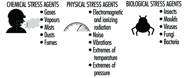
Figure 2. Observations and questions to ask on a walk-through survey.
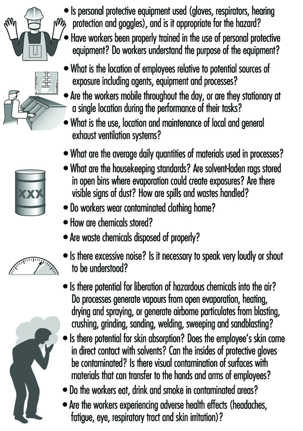
In addition to the questions shown in figure 5, questions should be asked that uncover what is not immediately obvious. Questions could address:
- non-routine tasks and schedules for maintenance and cleaning activities
- recent process changes and chemical substitutions
- recent physical changes in the work environment
- changes in job functions
- recent renovations and repairs.
Non-routine tasks can result in significant peak exposures to chemicals that are difficult to predict and measure during a typical workday. Process changes and chemical substitutions may alter the release of substances into the air and affect subsequent exposure. Changes in the physical layout of a work area can alter the effectiveness of an existing ventilation system. Changes in job functions can result in tasks performed by inexperienced workers and increased exposures. Renovations and repairs may introduce new materials and chemicals into the work environment which off-gas volatile organic chemicals or are irritants.
Indoor Air Quality Surveys
Indoor air quality surveys are distinct from traditional occupational hygiene surveys because they are typically encountered in non-industrial workplaces and may involve exposures to mixtures of trace quantities of chemicals, none of which alone appears capable of causing illness (Ness 1991). The goal of indoor air quality surveys is similar to occupational hygiene surveys in terms of identifying sources of contamination and determining the need for monitoring. However, indoor air quality surveys are always motivated by employee health complaints. In many cases, the employees have a variety of symptoms including headaches, throat irritation, lethargy, coughing, itching, nausea and non-specific hypersensitivity reactions that disappear when they go home. When health complaints do not disappear after the employees leave work, non-occupational exposures should be considered as well. Non-occupational exposures include hobbies, other jobs, urban air pollution, passive smoking and indoor exposures in the home. Indoor air quality surveys frequently use questionnaires to document employee symptoms and complaints and link them to job location or job function within the building. The areas with the highest incidence of symptoms are then targeted for further inspection.
Sources of indoor air contaminants that have been documented in indoor air quality surveys include:
- inadequate ventilation (52%)
- contamination from inside of the building (17%)
- contamination from outside of the building (11%)
- microbial contamination (5%)
- contamination from the building materials (3%)
- unknown causes (12%).
For indoor air quality investigations, the walk-through inspection is essentially a building and environmental inspection to determine potential sources of contamination both inside and outside of the building. Inside building sources include:
- building construction materials such as insulation, particleboard, adhesives and paints
- human occupants that can release chemicals from metabolic activities
- human activities such as smoking
- equipment such as copy machines
- ventilation systems that can be contaminated with micro-organisms.
Observations and questions that can be asked during the survey are listed in figure 3.
Figure 3. Observations and questions for an indoor air quality walk-through survey.
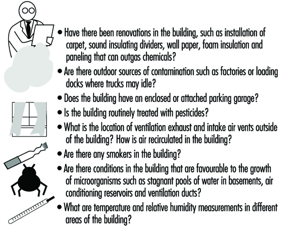
Sampling and Measurement Strategies
Occupational exposure limits
After the walk-through inspection is completed, the occupational hygienist must determine whether sampling is necessary; sampling should be performed only if the purpose is clear. The occupational hygienist must ask, “What will be made of the sampling results and what questions will the results answer?” It is relatively easy to sample and obtain numbers; it is far more difficult to interpret them.
Air and biological sampling data are usually compared to recommended or mandated occupational exposure limits (OELs). Occupational exposure limits have been developed in many countries for inhalation and biological exposure to chemical and physical agents. To date, out of a universe of over 60,000 commercially used chemicals, approximately 600 have been evaluated by a variety of organizations and countries. The philosophical bases for the limits are determined by the organizations that have developed them. The most widely used limits, called threshold limit values (TLVs), are those issued in the United States by the American Conference of Governmental Industrial Hygienists (ACGIH). Most of the OELs used by the Occupational Safety and Health Administration (OSHA) in the United States are based upon the TLVs. However, the National Institute for Occupational Safety and Health (NIOSH) of the US Department of Health and Human Services has suggested their own limits, called recommended exposure limits (RELs).
For airborne exposures, there are three types of TLVs: an eight-hour time-weighted-average exposure, TLV-TWA, to protect against chronic health effects; a fifteen-minute average short-term exposure limit, TLV-STEL, to protect against acute health effects; and an instantaneous ceiling value, TLV-C, to protect against asphyxiants or chemicals that are immediately irritating. Guidelines for biological exposure levels are called biological exposure indices (BEIs). These guidelines represent the concentration of chemicals in the body that would correspond to inhalation exposure of a healthy worker at a specific concentration in air. Outside of the United States as many as 50 countries or groups have established OELs, many of which are identical to the TLVs. In Britain, the limits are called the Health and Safety Executive Occupational Exposure Standards (OES), and in Germany OELs are called Maximum Workplace Concentrations (MAKs).
OELs have been set for airborne exposures to gases, vapours and particulates; they do not exist for airborne exposures to biological agents. Therefore, most investigations of bioaerosol exposure compare indoor with outdoor concentrations. If the indoor/outdoor profile and concentration of organisms is different, an exposure problem may exist. There are no OELs for skin and surface sampling, and each case must be evaluated separately. In the case of surface sampling, concentrations are usually compared with acceptable background concentrations that were measured in other studies or were determined in the current study. For skin sampling, acceptable concentrations are calculated based upon toxicity, rate of absorption, amount absorbed and total dose. In addition, biological monitoring of a worker may be used to investigate skin absorption.
Sampling strategy
An environmental and biological sampling strategy is an approach to obtaining exposure measurements that fulfils a purpose. A carefully designed and effective strategy is scientifically defensible, optimizes the number of samples obtained, is cost-effective and prioritizes needs. The goal of the sampling strategy guides decisions concerning what to sample (selection of chemical agents), where to sample (personal, area or source sample), whom to sample (which worker or group of workers), sample duration (real-time or integrated), how often to sample (how many days), how many samples, and how to sample (analytical method). Traditionally, sampling performed for regulatory purposes involves brief campaigns (one or two days) that concentrate on worst-case exposures. While this strategy requires a minimum expenditure of resources and time, it often captures the least amount of information and has little applicability to evaluating long-term occupational exposures. To evaluate chronic exposures so that they are useful for occupational physicians and epidemiological studies, sampling strategies must involve repeated sampling over time for large numbers of workers.
Purpose
The goal of environmental and biological sampling strategies is either to evaluate individual employee exposures or to evaluate contaminant sources. Employee monitoring may be performed to:
- evaluate individual exposures to chronic or acute toxicants
- respond to employee complaints about health and odours
- create a baseline of exposures for a long-term monitoring programme
- determine whether exposures comply with governmental regulations
- evaluate the effectiveness of engineering or process controls
- evaluate acute exposures for emergency response
- evaluate exposures at hazardous waste sites
- evaluate the impact of work practices on exposure
- evaluate exposures for individual job tasks
- investigate chronic illnesses such as lead and mercury poisoning
- investigate the relationship between occupational exposure and disease
- carry out an epidemiological study.
Source and ambient air monitoring may be performed to:
- establish a need for engineering controls such as local exhaust ventilation systems and enclosures
- evaluate the impact of equipment or process modifications
- evaluate the effectiveness of engineering or process controls
- evaluate emissions from equipment or processes
- evaluate compliance after remediation activities such as asbestos and lead removal
- respond to indoor air, community illness and odour complaints
- evaluate emissions from hazardous waste sites
- investigate an emergency response
- carry out an epidemiological study.
When monitoring employees, air sampling provides surrogate measures of dose resulting from inhalation exposure. Biological monitoring can provide the actual dose of a chemical resulting from all absorption routes including inhalation, ingestion, injection and skin. Thus, biological monitoring can more accurately reflect an individual’s total body burden and dose than air monitoring. When the relationship between airborne exposure and internal dose is known, biological monitoring can be used to evaluate past and present chronic exposures.
Goals of biological monitoring are listed in figure 4.
Figure 4. Goals of biological monitoring.
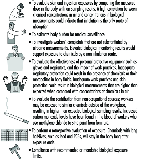
Biological monitoring has its limitations and should be performed only if it accomplishes goals that cannot be accomplished with air monitoring alone (Fiserova-Bergova 1987). It is invasive, requiring samples to be taken directly from workers. Blood samples generally provide the most useful biological medium to monitor; however, blood is taken only if non-invasive tests such as urine or exhaled breath are not applicable. For most industrial chemicals, data concerning the fate of chemicals absorbed by the body are incomplete or non-existent; therefore, only a limited number of analytical measurement methods are available, and many are not sensitive or specific.
Biological monitoring results may be highly variable between individuals exposed to the same airborne concentrations of chemicals; age, health, weight, nutritional status, drugs, smoking, alcohol consumption, medication and pregnancy can impact uptake, absorption, distribution, metabolism and elimination of chemicals.
What to sample
Most occupational environments have exposures to multiple contaminants. Chemical agents are evaluated both individually and as multiple simultaneous assaults on workers. Chemical agents can act independently within the body or interact in a way that increases the toxic effect. The question of what to measure and how to interpret the results depends upon the biological mechanism of action of the agents when they are within the body. Agents can be evaluated separately if they act independently on altogether different organ systems, such as an eye irritant and a neurotoxin. If they act on the same organ system, such as two respiratory irritants, their combined effect is important. If the toxic effect of the mixture is the sum of the separate effects of the individual components, it is termed additive. If the toxic effect of the mixture is greater than the sum of the effects of the separate agents, their combined effect is termed synergistic. Exposure to cigarette smoking and inhalation of asbestos fibres gives rise to a much greater risk of lung cancer than a simple additive effect.Sampling all the chemical agents in a workplace would be both expensive and not necessarily defensible. The occupational hygienist must prioritize the laundry list of potential agents by hazard or risk to determine which agents receive the focus.
Factors involved in ranking chemicals include:
- whether the agents interact independently, additively or synergistically
- inherent toxicity of the chemical agent
- quantities used and generated
- number of people potentially exposed
- anticipated duration and concentration of the exposure
- confidence in the engineering controls
- anticipated changes in the processes or controls
- occupational exposure limits and guidelines.
To provide the best estimate of employee exposure, air samples are taken in the breathing zone of the worker (within a 30 cm radius of the head), and are called personal samples. To obtain breathing zone samples, the sampling device is placed directly on the worker for the duration of the sampling. If air samples are taken near the worker, outside of the breathing zone, they are called area samples. Area samples tend to underestimate personal exposures and do not provide good estimates of inhalation exposure. However, area samples are useful for evaluating contaminant sources and measuring ambient levels of contaminants. Area samples can be taken while walking through the workplace with a portable instrument, or with fixed sampling stations. Area sampling is routinely used at asbestos abatement sites for clearance sampling and for indoor air investigations.
Whom to sample
Ideally, to evaluate occupational exposure, each worker would be individually sampled for multiple days over the course of weeks or months. However, unless the workplace is small (<10 employees), it is usually not feasible to sample all the workers. To minimize the sampling burden in terms of equipment and cost, and increase the effectiveness of the sampling programme, a subset of employees from the workplace is sampled, and their monitoring results are used to represent exposures for the larger work force.
To select employees who are representative of the larger work force, one approach is to classify employees into groups with similar expected exposures, called homogeneous exposure groups (HEGs) (Corn 1985). After the HEGs are formed, a subset of workers is randomly selected from each group for sampling. Methods for determining the appropriate sample sizes assume a lognormal distribution of exposures, an estimated mean exposure, and a geometric standard deviation of 2.2 to 2.5. Prior sampling data might allow a smaller geometric standard deviation to be used. To classify employees into distinct HEGs, most occupational hygienists observe workers at their jobs and qualitatively predict exposures.
There are many approaches to forming HEGs; generally, workers may be classified by job task similarity or work area similarity. When both job and work area similarity are used, the method of classification is called zoning (see figure 5). Once airborne, chemical and biological agents can have complex and unpredictable spatial and temporal concentration patterns throughout the work environment. Therefore, proximity of the source relative to the employee may not be the best indicator of exposure similarity. Exposure measurements made on workers initially expected to have similar exposures may show that there is more variation between workers than predicted. In these cases, the exposure groups should be reconstructed into smaller sets of workers, and sampling should continue to verify that workers within each group actually have similar exposures (Rappaport 1995).
Figure 5. Factors involved in creating HEGs using zoning.
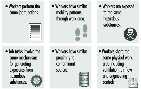
Exposures can be estimated for all the employees, regardless of job title or risk, or it can be estimated only for employees who are assumed to have the highest exposures; this is called worst-case sampling. The selection of worst-case sampling employees may be based upon production, proximity to the source, past sampling data, inventory and chemical toxicity. The worst-case method is used for regulatory purposes and does not provide a measure of long-term mean exposure and day-to-day variability. Task-related sampling involves selecting workers with jobs that have similar tasks that occur on a less than daily basis.
There are many factors that enter into exposure and can affect the success of HEG classification, including the following:
- Employees rarely perform the same work even when they have the same job description, and rarely have the same exposures.
- Employee work practices can significantly alter exposure.
- Workers who are mobile throughout the work area may be unpredictably exposed to several contaminant sources throughout the day.
- Air movement in a workplace can unpredictably increase the exposures of workers who are located a considerable distance from a source.
- Exposures may be determined not by the job tasks but by the work environment.
Sample duration
The concentrations of chemical agents in air samples are either measured directly in the field, obtaining immediate results (real-time or grab), or are collected over time in the field on sampling media or in sampling bags and are measured in a laboratory (integrated) (Lynch 1995). The advantage of real-time sampling is that results are obtained quickly onsite, and can capture measurements of short-term acute exposures. However, real-time methods are limited because they are not available for all contaminants of concern and they may not be analytically sensitive or accurate enough to quantify the targeted contaminants. Real-time sampling may not be applicable when the occupational hygienist is interested in chronic exposures and requires time-weighted-average measurements to compare with OELs.Real-time sampling is used for emergency evaluations, obtaining crude estimates of concentration, leak detection, ambient air and source monitoring, evaluating engineering controls, monitoring short-term exposures that are less than 15 minutes, monitoring episodic exposures, monitoring highly toxic chemicals (carbon monoxide), explosive mixtures and process monitoring. Real-time sampling methods can capture changing concentrations over time and provide immediate qualitative and quantitative information. Integrated air sampling is usually performed for personal monitoring, area sampling and for comparing concentrations to time-weighted-average OELs. The advantages of integrated sampling are that methods are available for a wide variety of contaminants; it can be used to identify unknowns; accuracy and specificity is high and limits of detection are usually very low. Integrated samples that are analysed in a laboratory must contain enough contaminant to meet minimum detectable analytical requirements; therefore, samples are collected over a predetermined time period.
In addition to analytical requirements of a sampling method, sample duration should be matched to the sampling purpose. For source sampling, duration is based upon the process or cycle time, or when there are anticipated peaks of concentrations. For peak sampling, samples should be collected at regular intervals throughout the day to minimize bias and identify unpredictable peaks. The sampling period should be short enough to identify peaks while also providing a reflection of the actual exposure period.
For personal sampling, duration is matched to the occupational exposure limit, task duration or anticipated biological effect. Real-time sampling methods are used for assessing acute exposures to irritants, asphyxiants, sensitizers and allergenic agents. Chlorine, carbon monoxide and hydrogen sulphide are examples of chemicals that can exert their effects quickly and at relatively low concentrations.
Chronic disease agents such as lead and mercury are usually sampled for a full shift (seven hours or more per sample), using integrated sampling methods. To evaluate full shift exposures, the occupational hygienist uses either a single sample or a series of consecutive samples that cover the entire shift. The sampling duration for exposures that occur for less than a full shift are usually associated with particular tasks or processes. Construction workers, indoor maintenance personnel and maintenance road crews are examples of jobs with exposures that are tied to tasks.
How many samples and how often to sample?
Concentrations of contaminants can vary minute to minute, day to day and season to season, and variability can occur between individuals and within an individual. Exposure variability affects both the number of samples and the accuracy of the results. Variations in exposure can arise from different work practices, changes in pollutant emissions, the volume of chemicals used, production quotas, ventilation, temperature changes, worker mobility and task assignments. Most sampling campaigns are performed for a couple of days in a year; therefore, the measurements obtained are not representative of exposure. The period over which samples are collected is very short compared with the unsampled period; the occupational hygienist must extrapolate from the sampled to the unsampled period. For long-term exposure monitoring, each worker selected from a HEG should be sampled multiple times over the course of weeks or months, and exposures should be characterized for all shifts. While the day shift may be the busiest, the night shift may have the least supervision and there may be lapses in work practices.
Measurement Techniques
Active and passive sampling
Contaminants are collected on sampling media either by actively pulling an air sample through the media, or by passively allowing the air to reach the media. Active sampling uses a battery-powered pump, and passive sampling uses diffusion or gravity to bring the contaminants to the sampling media. Gases, vapours, particulates and bioaerosols are all collected by active sampling methods; gases and vapours can also be collected by passive diffusion sampling.
For gases, vapours and most particulates, once the sample is collected the mass of the contaminant is measured, and concentration is calculated by dividing the mass by the volume of sampled air. For gases and vapours, concentration is expressed as parts per million (ppm) or mg/m3, and for particulates concentration is expressed as mg/m3 (Dinardi 1995).
In integrated sampling, air sampling pumps are critical components of the sampling system because concentration estimates require knowledge of the volume of sampled air. Pumps are selected based upon desired flowrate, ease of servicing and calibration, size, cost and suitability for hazardous environments. The primary selection criterion is flowrate: low-flow pumps (0.5 to 500 ml/min) are used for sampling gases and vapours; high-flow pumps (500 to 4,500 ml/min) are used for sampling particulates, bioaerosols and gases and vapours. To insure accurate sample volumes, pumps must be accurately calibrated. Calibration is performed using primary standards such as manual or electronic soap-bubble meters, which directly measure volume, or secondary methods such as wet test meters, dry gas meters and precision rotameters that are calibrated against primary methods.
Gases and vapours: sampling media
Gases and vapours are collected using porous solid sorbent tubes, impingers, passive monitors and bags. Sorbent tubes are hollow glass tubes that have been filled with a granular solid that enables adsorption of chemicals unchanged on its surface. Solid sorbents are specific for groups of compounds; commonly used sorbents include charcoal, silica gel and Tenax. Charcoal sorbent, an amorphous form of carbon, is electrically nonpolar, and preferentially adsorbs organic gases and vapours. Silica gel, an amorphous form of silica, is used to collect polar organic compounds, amines and some inorganic compounds. Because of its affinity for polar compounds, it will adsorb water vapour; therefore, at elevated humidity, water can displace the less polar chemicals of interest from the silica gel. Tenax, a porous polymer, is used for sampling very low concentrations of nonpolar volatile organic compounds.
The ability to accurately capture the contaminants in air and avoid contaminant loss depends upon the sampling rate, sampling volume, and the volatility and concentration of the airborne contaminant. Collection efficiency of solid sorbents can be adversely affected by increased temperature, humidity, flowrate, concentration, sorbent particle size and number of competing chemicals. As collection efficiency decreases chemicals will be lost during sampling and concentrations will be underestimated. To detect chemical loss, or breakthrough, solid sorbent tubes have two sections of granular material separated by a foam plug. The front section is used for sample collection and the back section is used to determine breakthrough. Breakthrough has occurred when at least 20 to 25% of the contaminant is present in the back section of the tube. Analysis of contaminants from solid sorbents requires extraction of the contaminant from the medium using a solvent. For each batch of sorbent tubes and chemicals collected, the laboratory must determine the desorption efficiency, the efficiency of removal of chemicals from the sorbent by the solvent. For charcoal and silica gel, the most commonly used solvent is carbon disulphide. For Tenax, the chemicals are extracted using thermal desorption directly into a gas chromatograph.
Impingers are usually glass bottles with an inlet tube that allows air to be drawn into the bottle through a solution that collects the gases and vapours by absorption either unchanged in solution or by a chemical reaction. Impingers are used less and less in workplace monitoring, especially for personal sampling, because they can break, and the liquid media can spill onto the employee. There are a variety of types of impingers, including gas wash bottles, spiral absorbers, glass bead columns, midget impingers and fritted bubblers. All impingers can be used to collect area samples; the most commonly used impinger, the midget impinger, can be used for personal sampling as well.
Passive, or diffusion monitors are small, have no moving parts and are available for both organic and inorganic contaminants. Most organic monitors use activated charcoal as the collection medium. In theory, any compound that can be sampled by a charcoal sorbent tube and pump can be sampled using a passive monitor. Each monitor has a uniquely designed geometry to give an effective sampling rate. Sampling starts when the monitor cover is removed and ends when the cover is replaced. Most diffusion monitors are accurate for eight-hour time-weighted-average exposures and are not appropriate for short-term exposures.
Sampling bags can be used to collect integrated samples of gases and vapours. They have permeability and adsorptive properties that enable storage for a day with minimal loss. Bags are made of Teflon (polytetrafluoroethylene) and Tedlar (polyvinylfluoride).
Sampling media: particulate materials
Occupational sampling for particulate materials, or aerosols, is currently in a state of flux; traditional sampling methods will eventually be replaced by particle size selective (PSS) sampling methods. Traditional sampling methods will be discussed first, followed by PSS methods.
The most commonly used media for collecting aerosols are fibre or membrane filters; aerosol removal from the air stream occurs by collision and attachment of the particles to the surface of the filters. The choice of filter medium depends upon the physical and chemical properties of the aerosols to be sampled, the type of sampler and the type of analysis. When selecting filters, they must be evaluated for collection efficiency, pressure drop, hygroscopicity, background contamination, strength and pore size, which can range from 0.01 to 10 μm. Membrane filters are manufactured in a variety of pore sizes and are usually made from cellulose ester, polyvinylchloride or polytetrafluoroethylene. Particle collection occurs at the surface of the filter; therefore, membrane filters are usually used in applications where microscopy will be performed. Mixed cellulose ester filters can be easily dissolved with acid and are usually used for collection of metals for analysis by atomic absorption. Nucleopore filters (polycarbonate) are very strong and thermally stable, and are used for sampling and analysing asbestos fibres using transmission electron microscopy. Fibre filters are usually made of fibreglass and are used to sample aerosols such as pesticides and lead.
For occupational exposures to aerosols, a known volume of air can be sampled through the filters, the total increase in mass (gravimetric analysis) can be measured (mg/m3 air), the total number of particles can be counted (fibres/cc) or the aerosols can be identified (chemical analysis). For mass calculations, the total dust that enters the sampler or only the respirable fraction can be measured. For total dust, the increase in mass represents exposure from deposition in all parts of the respiratory tract. Total dust samplers are subject to error due to high winds passing across the sampler and improper orientation of the sampler. High winds, and filters facing upright, can result in collection of extra particles and overestimation of exposure.
For respirable dust sampling, the increase in mass represents exposure from deposition in the gas exchange (alveolar) region of the respiratory tract. To collect only the respirable fraction, a preclassifier called a cyclone is used to alter the distribution of airborne dust presented to the filter. Aerosols are drawn into the cyclone, accelerated and whirled, causing the heavier particles to be thrown out to the edge of the air stream and dropped to a removal section at the bottom of the cyclone. The respirable particles that are less than 10 μm remain in the air stream and are drawn up and collected on the filter for subsequent gravimetric analysis.
Sampling errors encountered when performing total and respirable dust sampling result in measurements that do not accurately reflect exposure or relate to adverse health effects. Therefore, PSS has been proposed to redefine the relationship between particle size, adverse health impact and sampling method. In PSS sampling, the measurement of particles is related to the sizes that are associated with specific health effects. The International Organization for Standardization (ISO) and the ACGIH have proposed three particulate mass fractions: inhalable particulate mass (IPM), thoracic particulate mass (TPM) and respirable particulate mass (RPM). IPM refers to particles that can be expected to enter through the nose and mouth, and would replace the traditional total mass fraction. TPM refers to particles that can penetrate the upper respiratory system past the larynx. RPM refers to particles that are capable of depositing in the gas-exchange region of the lung, and would replace the current respirable mass fraction. The practical adoption of PSS sampling requires the development of new aerosol sampling methods and PSS-specific occupational exposure limits.
Sampling media: biological materials
There are few standardized methods for sampling biological material or bioaerosols. Although sampling methods are similar to those used for other airborne particulates, viability of most bioaerosols must be preserved to ensure laboratory culturability. Therefore, they are more difficult to collect, store and analyse. The strategy for sampling bioaerosols involves collection directly on semisolid nutrient agar or plating after collection in fluids, incubation for several days and identification and quantification of the cells that have grown. The mounds of cells that have multiplied on the agar can be counted as colony-forming units (CFU) for viable bacteria or fungi, and plaque-forming units (PFU) for active viruses. With the exception of spores, filters are not recommended for bioaerosol collection because dehydration causes cell damage.
Viable aerosolized micro-organisms are collected using all-glass impingers (AGI-30), slit samplers and inertial impactors. Impingers collect bioaerosols in liquid and the slit sampler collects bioaerosols on glass slides at high volumes and flowrates. The impactor is used with one to six stages, each containing a Petri dish, to allow for separation of particles by size.
Interpretation of sampling results must be done on a case-by-case basis because there are no occupational exposure limits. Evaluation criteria must be determined prior to sampling; for indoor air investigations, in particular, samples taken outside of the building are used as a background reference. A rule of thumb is that concentrations should be ten times background to suspect contamination. When using culture plating techniques, concentrations are probably underestimated because of losses of viability during sampling and incubation.
Skin and surface sampling
There are no standard methods for evaluating skin exposure to chemicals and predicting dose. Surface sampling is performed primarily to evaluate work practices and identify potential sources of skin absorption and ingestion. Two types of surface sampling methods are used to assess dermal and ingestion potential: direct methods, which involve sampling the skin of a worker, and indirect methods, which involve wipe sampling surfaces.
Direct skin sampling involves placing gauze pads on the skin to absorb chemicals, rinsing the skin with solvents to remove contaminants and using fluorescence to identify skin contamination. Gauze pads are placed on different parts of the body and are either left exposed or are placed under personal protective equipment. At the end of the workday the pads are removed and are analysed in the laboratory; the distribution of concentrations from different parts of the body are used to identify skin exposure areas. This method is inexpensive and easy to perform; however, the results are limited because gauze pads are not good physical models of the absorption and retention properties of skin, and measured concentrations are not necessarily representative of the entire body.
Skin rinses involve wiping the skin with solvents or placing hands in plastic bags filled with solvents to measure the concentration of chemicals on the surface. This method can underestimate dose because only the unabsorbed fraction of chemicals is collected.
Fluorescence monitoring is used to identify skin exposure for chemicals that naturally fluoresce, such as polynuclear aromatics, and to identify exposures for chemicals in which fluorescent compounds have been intentionally added. The skin is scanned with an ultraviolet light to visualize contamination. This visualization provides workers with evidence of the effect of work practices on exposure; research is underway to quantify the fluorescence intensity and relate it to dose.
Indirect wipe sampling methods involve the use of gauze, glass fibre filters or cellulose paper filters, to wipe the insides of gloves or respirators, or the tops of surfaces. Solvents may be added to increase collection efficiency. The gauze or filters are then analysed in the laboratory. To standardize the results and enable comparison between samples, a square template is used to sample a 100 cm2 area.
Biological media
Blood, urine and exhaled air samples are the most suitable specimens for routine biological monitoring, while hair, milk, saliva and nails are less frequently used. Biological monitoring is performed by collecting bulk blood and urine samples in the workplace and analysing them in the laboratory. Exhaled air samples are collected in Tedlar bags, specially designed glass pipettes or sorbent tubes, and are analysed in the field using direct-reading instruments, or in the laboratory. Blood, urine and exhaled air samples are primarily used to measure the unchanged parent compound (same chemical that is sampled in workplace air), its metabolite or a biochemical change (intermediate) that has been induced in the body. For example, the parent compound lead is measured in blood to evaluate lead exposure, the metabolite mandelic acid is measured in urine for both styrene and ethyl benzene, and carboxyhaemoglobin is the intermediate measured in blood for both carbon monoxide and methylene chloride exposure. For exposure monitoring, the concentration of an ideal determinant will be highly correlated with intensity of exposure. For medical monitoring, the concentration of an ideal determinant will be highly correlated with target organ concentration.
The timing of specimen collection can impact the usefulness of the measurements; samples should be collected at times which most accurately reflect exposure. Timing is related to the excretion biological half-life of a chemical, which reflects how quickly a chemical is eliminated from the body; this can vary from hours to years. Target organ concentrations of chemicals with short biological half-lives closely follow the environmental concentration; target organ concentrations of chemicals with long biological half-lives fluctuate very little in response to environmental exposures. For chemicals with short biological half-lives, less than three hours, a sample is taken immediately at the end of the workday, before concentrations rapidly decline, to reflect exposure on that day. Samples may be taken at any time for chemicals with long half-lives, such as polychlorinated biphenyls and lead.
Real-time monitors
Direct-reading instruments provide real-time quantification of contaminants; the sample is analysed within the equipment and does not require off-site laboratory analysis (Maslansky and Maslansky 1993). Compounds can be measured without first collecting them on separate media, then shipping, storing and analysing them. Concentration is read directly from a meter, display, strip chart recorder and data logger, or from a colour change. Direct-reading instruments are primarily used for gases and vapours; a few instruments are available for monitoring particulates. Instruments vary in cost, complexity, reliability, size, sensitivity and specificity. They include simple devices, such as colorimetric tubes, that use a colour change to indicate concentration; dedicated instruments that are specific for a chemical, such as carbon monoxide indicators, combustible gas indicators (explosimeters) and mercury vapour meters; and survey instruments, such as infrared spectrometers, that screen large groups of chemicals. Direct-reading instruments use a variety of physical and chemical methods to analyse gases and vapours, including conductivity, ionization, potentiometry, photometry, radioactive tracers and combustion.
Commonly used portable direct-reading instruments include battery-powered gas chromatographs, organic vapour analysers and infrared spectrometers. Gas chromatographs and organic vapour monitors are primarily used for environmental monitoring at hazardous waste sites and for community ambient air monitoring. Gas chromatographs with appropriate detectors are specific and sensitive, and can quantify chemicals at very low concentrations. Organic vapour analysers are usually used to measure classes of compounds. Portable infrared spectrometers are primarily used for occupational monitoring and leak detection because they are sensitive and specific for a wide range of compounds.
Small direct-reading personal monitors are available for a few common gases (chlorine, hydrogen cyanide, hydrogen sulphide, hydrazine, oxygen, phosgene, sulphur dioxide, nitrogen dioxide and carbon monoxide). They accumulate concentration measurements over the course of the day and can provide a direct readout of time-weighted-average concentration as well as provide a detailed contaminant profile for the day.
Colorimetric tubes (detector tubes) are simple to use, cheap and available for a wide variety of chemicals. They can be used to quickly identify classes of air contaminants and provide ballpark estimates of concentrations that can be used when determining pump flow rates and volumes. Colorimetric tubes are glass tubes filled with solid granular material which has been impregnated with a chemical agent that can react with a contaminant and create a colour change. After the two sealed ends of a tube are broken open, one end of the tube is placed in a hand pump. The recommended volume of contaminated air is sampled through the tube by using a specified number of pump strokes for a particular chemical. A colour change or stain is produced on the tube, usually within two minutes, and the length of the stain is proportional to concentration. Some colorimetric tubes have been adapted for long duration sampling, and are used with battery-powered pumps that can run for at least eight hours. The colour change produced represents a time-weighted-average concentration. Colorimetric tubes are good for both qualitative and quantitative analysis; however, their specificity and accuracy is limited. The accuracy of colorimetric tubes is not as high as that of laboratory methods or many other real-time instruments. There are hundreds of tubes, many of which have cross-sensitivities and can detect more than one chemical. This can result in interferences that modify the measured concentrations.
Direct-reading aerosol monitors cannot distinguish between contaminants, are usually used for counting or sizing particles, and are primarily used for screening, not to determine TWA or acute exposures. Real-time instruments use optical or electrical properties to determine total and respirable mass, particle count and particle size. Light-scattering aerosol monitors, or aerosol photometers, detect the light scattered by particles as they pass through a volume in the equipment. As the number of particles increases, the amount of scattered light increases and is proportional to mass. Light-scattering aerosol monitors cannot be used to distinguish between particle types; however, if they are used in a workplace where there are a limited number of dusts present, the mass can be attributed to a particular material. Fibrous aerosol monitors are used to measure the airborne concentration of particles such as asbestos. Fibres are aligned in an oscillating electric field and are illuminated with a helium neon laser; the resulting pulses of light are detected by a photomultiplier tube. Light-attenuating photometers measure the extinction of light by particles; the ratio of incident light to measured light is proportional to concentration.
Analytical Techniques
There are many available methods for analysing laboratory samples for contaminants. Some of the more commonly used techniques for quantifying gases and vapours in air include gas chromatography, mass spectrometry, atomic absorption, infrared and UV spectroscopy and polarography.
Gas chromatography is a technique used to separate and concentrate chemicals in mixtures for subsequent quantitative analysis. There are three main components to the system: the sample injection system, a column and a detector. A liquid or gaseous sample is injected using a syringe, into an air stream that carries the sample through a column where the components are separated. The column is packed with materials that interact differently with different chemicals, and slows down the movement of the chemicals. The differential interaction causes each chemical to travel through the column at a different rate. After separation, the chemicals go directly into a detector, such as a flame ionization detector (FID), photo-ionization detector (PID) or electron capture detector (ECD); a signal proportional to concentration is registered on a chart recorder. The FID is used for almost all organics including: aromatics, straight chain hydrocarbons, ketones and some chlorinated hydrocarbons. Concentration is measured by the increase in the number of ions produced as a volatile hydrocarbon is burned by a hydrogen flame. The PID is used for organics and some inorganics; it is especially useful for aromatic compounds such as benzene, and it can detect aliphatic, aromatic and halogenated hydrocarbons. Concentration is measured by the increase in the number of ions produced when the sample is bombarded by ultraviolet radiation. The ECD is primarily used for halogen-containing chemicals; it gives a minimal response to hydrocarbons, alcohols and ketones. Concentration is measured by the current flow between two electrodes caused by ionization of the gas by radioactivity.
The mass spectrophotometer is used to analyse complex mixtures of chemicals present in trace amounts. It is often coupled with a gas chromatograph for the separation and quantification of different contaminants.
Atomic absorption spectroscopy is primarily used for the quantification of metals such as mercury. Atomic absorption is the absorption of light of a particular wavelength by a free, ground-state atom; the quantity of light absorbed is related to concentration. The technique is highly specific, sensitive and fast, and is directly applicable to approximately 68 elements. Detection limits are in the sub-ppb to low-ppm range.
Infrared analysis is a powerful, sensitive, specific and versatile technique. It uses the absorption of infrared energy to measure many inorganic and organic chemicals; the amount of light absorbed is proportional to concentration. The absorption spectrum of a compound provides information enabling its identification and quantification.
UV absorption spectroscopy is used for analysis of aromatic hydrocarbons when interferences are known to be low. The amount of absorption of UV light is directly proportional to concentration.
Polarographic methods are based upon the electrolysis of a sample solution using an easily polarized electrode and a nonpolarizable electrode. They are used for qualitative and quantitative analysis of aldehydes, chlorinated hydrocarbons and metals.
" DISCLAIMER: The ILO does not take responsibility for content presented on this web portal that is presented in any language other than English, which is the language used for the initial production and peer-review of original content. Certain statistics have not been updated since the production of the 4th edition of the Encyclopaedia (1998)."