Management of Air Pollution
The objective of a manager of an air pollution control system is to ensure that excessive concentrations of air pollutants do not reach a susceptible target. Targets could include people, plants, animals and materials. In all cases we should be concerned with the most sensitive of each of these groups. Air pollutants could include gases, vapours, aerosols and, in some cases, biohazardous materials. A well designed system will prevent a target from receiving a harmful concentration of a pollutant.
Most air pollution control systems involve a combination of several control techniques, usually a combination of technological controls and administrative controls, and in larger or more complex sources there may be more than one type of technological control.
Ideally, the selection of the appropriate controls will be made in the context of the problem to be solved.
- What is emitted, in what concentration?
- What are the targets? What is the most susceptible target?
- What are acceptable short-term exposure levels?
- What are acceptable long-term exposure levels?
- What combination of controls must be selected to ensure that the short-term and long-term exposure levels are not exceeded?
Table 1 describes the steps in this process.
Table 1. Steps in selecting pollution controls
|
Step 1: |
The first part is to determine what will be released from the stack. |
|
Step 2: |
All susceptible targets should be identified. This includes people, animals, plants and materials. In each case, the most susceptible member of each group must be identified. For example, asthmatics near a plant that emits isocyanates. |
|
Step 3: |
An acceptable level of exposure for the most sensitive target group must |
|
Step 4: |
Step 1 identifies the emissions, and Step 3 determines the acceptable |
* When setting exposure levels in Step 3, it must be remembered that these exposures are total exposures, not just those from the plant. Once the acceptable level has been established, background levels, and contributions from other plants just be subtracted to determine the maximum amount that the plant can emit without exceeding the acceptable exposure level. If this is not done, and three plants are allowed to emit at the maximum amount, the target groups will be exposed to three times the acceptable level.
** Some materials such as carcinogens do not have a threshold below which no harmful effects will occur. Therefore, as long as some of the material is allowed to escape to the environment, there will be some risk to the target populations. In this case a no effect level cannot be set (other than zero). Instead, an acceptable level of risk must be established. Usually this is set in the range of 1 adverse outcome in 100,000 to 1,000,000 exposed persons.
Some jurisdictions have done some of the work by setting standards based on the maximum concentration of a contaminant that a susceptible target can receive. With this type of standard, the manager does not have to carry out Steps 2 and 3, since the regulating agency has already done this. Under this system, the manager must establish only the uncontrolled emission standards for each pollutant (Step 1), and then determine what controls are necessary to meet the standard (Step 4).
By having air quality standards, regulators can measure individual exposures and thus determine whether anyone is exposed to potentially harmful levels. It is assumed that the standards set under these conditions are low enough to protect the most susceptible target group. This is not always a safe assumption. As shown in table 2, there can be a wide variation in common air quality standards. Air quality standards for sulphur dioxide range from 30 to 140 μg/m3. For less commonly regulated materials this variation can be even larger (1.2 to 1,718 μg/m3), as shown in table 3 for benzene. This is not surprising given that economics can play as large a role in standard setting as does toxicology. If a standard is not set low enough to protect susceptible populations, no one is well served. Exposed populations have a feeling of false confidence, and can unknowingly be put at risk. The emitter may at first feel that they have benefited from a lenient standard, but if effects in the community require the company to redesign their controls, or install new controls, costs could be higher than doing it correctly the first time.
Table 2. Range of air quality standards for a commonly controlled air contaminant (sulphur dioxide)
|
Countries and territories |
Long-term sulphur dioxide |
|
Australia |
50 |
|
Canada |
30 |
|
Finland |
40 |
|
Germany |
140 |
|
Hungary |
70 |
|
Taiwan |
133 |
Table 3. Range of air quality standards for a less commonly controlled air contaminant (benzene)
|
City/State |
24-hour air quality standard for |
|
Connecticut |
53.4 |
|
Massachusetts |
1.2 |
|
Michigan |
2.4 |
|
North Carolina |
2.1 |
|
Nevada |
254 |
|
New York |
1,718 |
|
Philadelphia |
1,327 |
|
Virginia |
300 |
The levels were standardized to an averaging time of 24 hours to assist in the comparisons.
(Adapted from Calabrese and Kenyon 1991.)
Sometimes this stepwise approach to selecting air pollution controls is short circuited, and the regulators and designers go directly to a “universal solution”. One such method is best available control technology (BACT). It is assumed that by using the best combination of scrubbers, filters and good work practices on an emission source, a level of emissions low enough to protect the most susceptible target group would be achieved. Frequently, the resulting emission level will be below the minimum required to protect the most susceptible targets. This way all unnecessary exposures should be eliminated. Examples of BACT are shown in table 4.
Table 4. Selected examples of best available control technology (BACT) showing the control method used and estimated efficiency
|
Process |
Pollutant |
Control method |
Estimated efficiency |
|
Soil remediation |
Hydrocarbons |
Thermal oxidizer |
99 |
|
Kraft pulp mill |
Particulates |
Electrostatic |
99.68 |
|
Production of fumed |
Carbon monoxide |
Good practice |
50 |
|
Automobile painting |
Hydrocarbons |
Oven afterburner |
90 |
|
Electric arc furnace |
Particulates |
Baghouse |
100 |
|
Petroleum refinery, |
Respirable particulates |
Cyclone + Venturi |
93 |
|
Medical incinerator |
Hydrogen chloride |
Wet scrubber + dry |
97.5 |
|
Coal-fired boiler |
Sulphur dioxide |
Spray dryer + |
90 |
|
Waste disposal by |
Particulates |
Cyclone + condenser |
95 |
|
Asphalt plant |
Hydrocarbons |
Thermal oxidizer |
99 |
BACT by itself does not ensure adequate control levels. Although this is the best control system based on gas cleaning controls and good operating practices, BACT may not be good enough if the source is a large plant, or if it is located next to a sensitive target. Best available control technology should be tested to ensure that it is indeed good enough. The resulting emission standards should be checked to determine whether or not they may still be harmful even with the best gas cleaning controls. If emission standards are still harmful, other basic controls, such as selecting safer processes or materials, or relocating in a less sensitive area, may have to be considered.
Another “universal solution” that bypasses some of the steps is source performance standards. Many jurisdictions establish emission standards that cannot be exceeded. Emission standards are based on emissions at the source. Usually this works well, but like BACT they can be unreliable. The levels should be low enough to maintain the maximum emissions low enough to protect susceptible target populations from typical emissions. However, as with best available control technology, this may not be good enough to protect everyone where there are large emission sources or nearby susceptible populations. If this is the case, other procedures must be used to ensure the safety of all target groups.
Both BACT and emission standards have a basic fault. They assume that if certain criteria are met at the plant, the target groups will be automatically protected. This is not necessarily so, but once such a system is passed into law, effects on the target become secondary to compliance with the law.
BACT and source emission standards or design criteria should be used as minimum criteria for controls. If BACT or emission criteria will protect the susceptible targets, then they can be used as intended, otherwise other administrative controls must be used.
Control Measures
Controls can be divided into two basic types of controls - technological and administrative. Technological controls are defined here as the hardware put on an emission source to reduce contaminants in the gas stream to a level that is acceptable to the community and that will protect the most sensitive target. Administrative controls are defined here as other control measures.
Technological controls
Gas cleaning systems are placed at the source, before the stack, to remove contaminants from the gas stream before releasing it to the environment. Table 5 shows a brief summary of the different classes of gas cleaning system.
Table 5. Gas cleaning methods for removing harmful gases, vapours and particulates from industrial process emissions
|
Control method |
Examples |
Description |
Efficiency |
|
Gases/Vapours |
|||
|
Condensation |
Contact condensers |
The vapour is cooled and condensed to a liquid. This is inefficient and is used as a preconditioner to other methods |
80+% when concentration >2,000 ppm |
|
Absorption |
Wet scrubbers (packed |
The gas or vapour is collected in a liquid. |
82–95% when concentration <100 ppm |
|
Adsorption |
Carbon |
The gas or vapour is collected on a solid. |
90+% when concentration <1,000 ppm |
|
Incineration |
Flares |
An organic gas or vapour is oxidized by heating it to a high temperature and holding it at that temperature for a |
Not recommended when |
|
Particulates |
|||
|
Inertial |
Cyclones |
Particle-laden gases are forced to change direction. The inertia of the particle causes them to separate from the gas stream. This is inefficient and is used as a |
70–90% |
|
Wet scrubbers |
Venturi |
Liquid droplets (water) collect the particles by impaction, interception and diffusion. The droplets and their particles are then separated from the gas stream. |
For 5 μm particles, 98.5% at 6.8 w.g.; |
|
Electrostatic |
Plate-wire |
Electrical forces are used to move the particles out of the gas stream onto collection plates |
95–99.5% for 0.2 μm particles |
|
Filters |
Baghouse |
A porous fabric removes particulates from the gas stream. The porous dust cake that forms on the fabric then actually |
99.9% for 0.2 μm particles |
The gas cleaner is part of a complex system consisting of hoods, ductwork, fans, cleaners and stacks. The design, performance and maintenance of each part affects the performance of all other parts, and the system as a whole.
It should be noted that system efficiency varies widely for each type of cleaner, depending on its design, energy input and the characteristics of the gas stream and the contaminant. As a result, the sample efficiencies in table 5 are only approximations. The variation in efficiencies is demonstrated with wet scrubbers in table 5. Wet scrubber collection efficiency goes from 98.5 per cent for 5 μm particles to 45 per cent for 1 μm particles at the same pressure drop across the scrubber (6.8 in. water gauge (w.g.)). For the same size particle, 1 μm, efficiency goes from 45 per cent efficiency at 6.8 w.g. to 99.95 at 50 w.g. As a result, gas cleaners must be matched to the specific gas stream in question. The use of generic devices is not recommended.
Waste disposal
When selecting and designing gas cleaning systems, careful consideration must be given to the safe disposal of the collected material. As shown in table 6, some processes produce large amounts of contaminants. If most of the contaminants are collected by the gas cleaning equipment there can be a hazardous waste disposal problem.
Table 6. Sample uncontrolled emission rates for selected industrial processes
|
Industrial source |
Emission rate |
|
100 ton electric furnace |
257 tons/year particulates |
|
1,500 MM BTU/hr oil/gas turbine |
444 lb/hr SO2 |
|
41.7 ton/hr incinerator |
208 lb/hr NOx |
|
100 trucks/day clear coat |
3,795 lb/week organics |
In some cases the wastes may contain valuable products that can be recycled, such as heavy metals from a smelter, or solvent from a painting line. The wastes can be used as a raw material for another industrial process - for example, sulphur dioxide collected as sulphuric acid can be used in the manufacture of fertilizers.
Where the wastes cannot be recycled or reused, disposal may not be simple. Not only can the volume be a problem, but they may be hazardous themselves. For example, if the sulphuric acid captured from a boiler or smelter cannot be reused, it will have to be further treated to neutralize it before disposal.
Dispersion
Dispersion can reduce the concentration of a pollutant at a target. However, it must be remembered that dispersion does not reduce the total amount of material leaving a plant. A tall stack only allows the plume to spread out and be diluted before it reaches ground level, where susceptible targets are likely to exist. If the pollutant is primarily a nuisance, such as an odour, dispersion may be acceptable. However if the material is persistent or cumulative, such as heavy metals, dilution may not be an answer to an air pollution problem.
Dispersion should be used with caution. Local meteorological and ground surface conditions must be taken into consideration. For example, in colder climates, particularly with snow cover, there can be frequent temperature inversions that can trap pollutants close to the ground, resulting in unexpectedly high exposures. Similarly, if a plant is located in a valley, the plumes may move up and down the valley, or be blocked by surrounding hills so that they do not spread out and disperse as expected.
Administrative controls
In addition to the technological systems, there is another group of controls that must be considered in the overall design of an air pollution control system. For the large part, they come from the basic tools of industrial hygiene.
Substitution
One of the preferred occupational hygiene methods for controlling environmental hazards in the workplace is to substitute a safer material or process. If a safer process or material can be used, and harmful emissions avoided, the type or efficacy of controls becomes academic. It is better to avoid the problem than it is to try to correct a bad first decision. Examples of substitution include the use of cleaner fuels, covers for bulk storage and reduced temperatures in dryers.
This applies to minor purchases as well as the major design criteria for the plant. If only environmentally safe products or processes are purchased, there will be no risk to the environment, indoors or out. If the wrong purchase is made, the remainder of the programme consists of trying to compensate for that first decision. If a low-cost but hazardous product or process is purchased it may need special handling procedures and equipment, and special disposal methods. As a result, the low-cost item may have only a low purchase price, but a high price to use and dispose of it. Perhaps a safer but more expensive material or process would have been less costly in the long run.
Local ventilation
Controls are required for all the identified problems that cannot be avoided by substituting safer materials or methods. Emissions start at the individual worksite, not the stack. A ventilation system that captures and controls emissions at the source will help protect the community if it is properly designed. The hoods and ducts of the ventilation system are part of the total air pollution control system.
A local ventilation system is preferred. It does not dilute the contaminants, and provides a concentrated gas stream that is easier to clean before release to the environment. Gas cleaning equipment is more efficient when cleaning air with higher concentrations of contaminants. For example, a capture hood over the pouring spout of a metal furnace will prevent contaminants from getting into the environment, and deliver the fumes to the gas cleaning system. In table 5 it can be seen that cleaning efficiencies for absorption and adsorption cleaners increase with the concentration of the contaminant, and condensation cleaners are not recommended for low levels (<2,000 ppm) of contaminants.
If pollutants are not caught at the source and are allowed to escape through windows and ventilation openings, they become uncontrolled fugitive emissions. In some cases, these uncontrolled fugitive emissions can have a significant impact on the immediate neighbourhood.
Isolation
Isolation - locating the plant away from susceptible targets - can be a major control method when engineering controls are inadequate by themselves. This may be the only means of achieving an acceptable level of control when best available control technology (BACT) must be relied on. If, after applying the best available controls, a target group is still at risk, consideration must be given to finding an alternate site where sensitive populations are not present.
Isolation, as presented above, is a means of separating an individual plant from susceptible targets. Another isolation system is where local authorities use zoning to separate classes of industries from susceptible targets. Once industries have been separated from target populations, the population should not be allowed to relocate next to the facility. Although this seems like common sense, it isn’t employed as often as it should be.
Work procedures
Work procedures must be developed to ensure that equipment is used properly and safely, without risk to workers or the environment. Complex air pollution systems must be properly maintained and operated if they are to do their job as intended. An important factor in this is staff training. Staff must be trained in how to use and maintain the equipment to reduce or eliminate the amount of hazardous materials emitted to the workplace or the community. In some cases BACT relies on good practice to ensure acceptable results.
Real time monitoring
A system based on real time monitoring is not popular, and is not commonly used. In this case, continuous emission and meteorological monitoring can be combined with dispersion modelling to predict downwind exposures. When the predicted exposures approach the acceptable levels, the information is used to reduce production rates and emissions. This is an inefficient method, but may be an acceptable interim control method for an existing facility.
The converse of this to announce warnings to the public when conditions are such that excessive concentrations of contaminants may exist, so that the public can take appropriate action. For example, if a warning is sent out that atmospheric conditions are such that sulphur dioxide levels downwind of a smelter are excessive, susceptible populations such as asthmatics would know not to go outside. Again, this may be an acceptable interim control until permanent controls are installed.
Real time atmospheric and meteorological monitoring is sometimes used to avoid or reduce major air pollution events where multiple sources may exist. When it becomes evident that excessive air pollution levels are likely, the personal use of cars may be restricted and major emitting industries shut down.
Maintenance/housekeeping
In all cases the effectiveness of the controls depends on proper maintenance; the equipment has to operate as intended. Not only must the air pollution controls be maintained and used as intended, but the processes generating potential emissions must be maintained and operated properly. An example of an industrial process is a wood chip dryer with a failing temperature controller; if the dryer is operated at too high a temperature, it will emit more materials, and perhaps a different type of material, from the drying wood. An example of gas cleaner maintenance affecting emissions would be a poorly maintained baghouse with broken bags, which would allow particulates to pass through the filter.
Housekeeping also plays an important part in controlling total emissions. Dusts that are not quickly cleaned up inside the plant can become re-entrained and present a hazard to staff. If the dusts are carried outside of the plant, they are a community hazard. Poor housekeeping in the plant yard could present a significant risk to the community. Uncovered bulk materials, plant wastes or vehicle-raised dusts can result in pollutants being carried on the winds into the community. Keeping the yard clean, using proper containers or storage sites, is important in reducing total emissions. A system must be not only designed properly, but used properly as well if the community is to be protected.
A worst case example of poor maintenance and housekeeping would be the lead recovery plant with a broken lead dust conveyor. The dust was allowed to escape from the conveyor until the pile was so high the dust could slide down the pile and out a broken window. Local winds then carried the dust around the neighbourhood.
Equipment for Emission Sampling
Source sampling can be carried out for several reasons:
- To characterize the emissions. To design an air pollution control system, one must know what is being emitted. Not only the volume of gas, but the amount, identity and, in the case of particulates, size distribution of the material being emitted must be known. The same information is necessary to catalogue total emissions in a neighbourhood.
- To test equipment efficiency. After an air pollution control system has been purchased, it should be tested to ensure that it is doing the intended job.
- As part of a control system. When emissions are continuously monitored, the data can be used to fine tune the air pollution control system, or the plant operation itself.
- To determine compliance. When regulatory standards include emission limits, emission sampling can be used to determine compliance or non-compliance with the standards.
The type of sampling system used will depend on the reason for taking the samples, costs, availability of technology, and training of staff.
Visible emissions
Where there is a desire to reduce the soiling power of the air, improve visibility or prevent the introduction of aerosols into the atmosphere, standards may be based on visible emissions.
Visible emissions are composed of small particles or coloured gases. The more opaque a plume is, the more material is being emitted. This characteristic is evident to the sight, and trained observers can be used to assess emission levels. There are several advantages to using this method of assessing emission standards:
- No expensive equipment is required.
- One person can make many observations in a day.
- Plant operators can quickly assess the effects of process changes at low cost.
- Violators can be cited without time-consuming source testing.
- Questionable emissions can be located and the actual emissions then determined by source testing as described in the following sections.
Extractive sampling
A much more rigorous sampling method calls for a sample of the gas stream to be removed from the stack and analysed. Although this sounds simple, it does not translate into a simple sampling method.
The sample should be collected isokinetically, especially when particulates are being collected. Isokinetic sampling is defined as sampling by drawing the sample into the sampling probe at the same velocity that the material is moving in the stack or duct. This is done by measuring the velocity of the gas stream with a pitot tube and then adjusting the sampling rate so that the sample enters the probe at the same velocity. This is essential when sampling for particulates, since larger, heavier particles will not follow a change in direction or velocity. As a result the concentration of larger particles in the sample will not be representative of the gas stream and the sample will be inaccurate.
A sample train for sulphur dioxide is shown in figure 1. It is not simple, and a trained operator is required to ensure that a sample is collected properly. If something other than sulphur dioxide is to be sampled, the impingers and ice bath can be removed and the appropriate collection device inserted.
Figure 1. A diagram of an isokinetic sampling train for sulphur dioxide
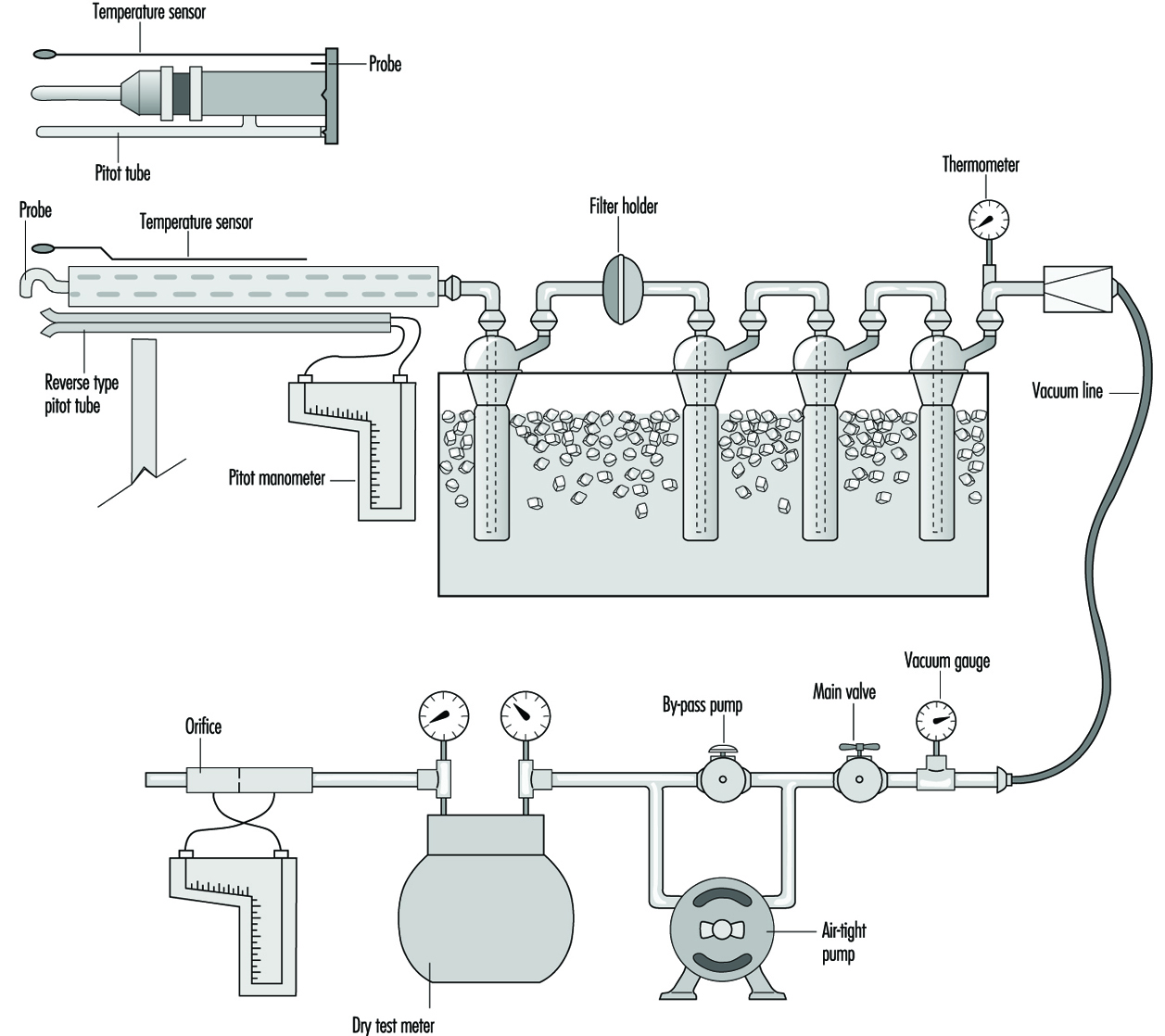
Extractive sampling, particularly isokinetic sampling, can be very accurate and versatile, and has several uses:
- It is a recognized sampling method with adequate quality controls, and thus can be used to determine compliance with standards.
- The potential accuracy of the method makes it suitable for performance testing of new control equipment.
- Since samples can be collected and analysed under controlled laboratory conditions for many components, it is useful for characterizing the gas stream.
A simplified and automated sampling system can be connected to a continuous gas (electrochemical, ultraviolet-photometric or flame ionization sensors) or particulate (nephelometer) analyzer to continuously monitor emissions. This can provide documentation of the emissions, and instantaneous operating status of the air pollution control system.
In situ sampling
Emissions can also be sampled in the stack. Figure 2 is a representation of a simple transmissometer used to measure materials in the gas stream. In this example, a beam of light is projected across the stack to a photocell. The particulates or coloured gas will absorb or block some of the light. The more material, the less light will get to the photocell. (See figure 2.)
Figure 2. A simple transmissometer to measure particulates in a stack
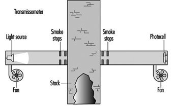
By using different light sources and detectors such as ultraviolet light (UV), gases transparent to visible light can be detected. These devices can be tuned to specific gases, and thus can measure gas concentration in the waste stream.
An in situ monitoring system has an advantage over an extractive system in that it can measure the concentration across the entire stack or duct, whereas the extractive method measures concentrations only at the point from which the sample was extracted. This can result in significant error if the sample gas stream is not well mixed. However, the extractive method offers more methods of analysis, and thus perhaps can be used in more applications.
Since the in situ system provides a continuous readout, it can be used to document emissions, or to fine tune the operating system.